Chapter 9. Data-Flow Analysis

ABSTRACT

Compilers analyze the IR form of the program in order to identify opportunities where the code can be improved and to prove the safety and profitability of transformations that might improve that code. Data-flow analysis is the classic technique for compile-time program analysis. It allows the compiler to reason about the runtime flow of values in the program.

This chapter explores iterative data-flow analysis, based on a simple fixed-point algorithm. From basic data-flow analysis, it builds up to construction of static single-assignment (ssa) form, illustrates the use of ssa form, and introduces interprocedural analysis.

KEYWORDS Data-Flow Analysis, Dominance, Static Single-Assignment Form, Constant Propagation

9.1 Introduction

As we saw in Chapter $8$, optimization is the process of analyzing a program and transforming it in ways that improve its runtime behavior. Before the compiler can improve the code, it must locate points in the program where changing the code is likely to provide improvement, and it must prove that changing the code at those points is safe. Both of these tasks require a deeper understanding of the code than the compiler's front end typically derives. To gather the information needed to find opportunities for optimization and to justify those optimizations, compilers use some form of static analysis.

In general, static analysis involves compile-time reasoning about the runtime flow of values. This chapter explores techniques that compilers use to analyze programs in support of optimization.

Conceptual Roadmap

Compilers use static analysis to determine where optimizing transformations can be safely and profitably applied. In Chapter $8$, we saw that optimizations operate on different scopes, from local to interprocedural. Ingeneral, a transformation needs analytical information that covers at least as large a scope as the transformation; that is, a local optimization needs at least local information, while a whole-procedure, or global, optimization needs global information.

Static analysis generally begins with control-flow analysis; the compiler builds a graph that represents the flow of control within the code. Next, the compiler analyzes the details of how values flow through the code. It uses the resulting information to find opportunities for improvement and to prove the safety of transformations. Data-flow analysis was developed to answer these questions.

Static single-assignment (SSA) form is an intermediate representation that unifies the results of control-flow and data-flow analysis in a single sparse data structure. It has proven useful in both analysis and transformation and has become a standard ir used in both research and production compilers.

Overview

Chapter 8 introduced the subject of analysis and transformation of programs by examining local methods, regional methods, global methods, and interprocedural methods. Value numbering is algorithmically simple, even though it achieves complex effects; it finds redundant expressions, simplifies code based on algebraic identities and zero, and propagates known constant values. By contrast, finding an uninitialized variable is conceptually simple, but it requires the compiler to analyze the entire procedure to track definitions and uses.

Join point In a CFG, a join point is a node that has multiple predecessors.

The difference in complexity between these two problems lies in the kinds of control flows that they encounter. Local and superlocal value numbering deal with subsets of the control-flow graph (CFG) that form trees (see Sections 8.4.1 and 8.5.1). To analyze the entire procedure, the compiler must reason about the full cfg, including cycles and join points, which both complicate analysis. In general, methods that only handle acyclic subsets of the cfg are amenable to online solutions, while those that deal with cycles in the cfg require offline solutions--the entire analysis must complete before rewriting can begin.

Static analysis analysis performed at compile time or link time

Dynamic analysis analysis performed at runtime, perhaps in a JIT or specialized self-modifying code

Static analysis, or compile-time analysis, is a collection of techniques that compilers use to prove the safety and profitability of a potential transformation. Static analysis over single blocks or trees of blocks is typically straightforward. This chapter focuses on global analysis, where the cfg can contain both cycles and join points. It mentions several problems in interprocedural analysis; these problems operate over the program's call graph or some related graph.

In simple cases, static analysis can produce precise results--the compiler can know exactly what will happen when the code executes. If the compiler can derive precise information, it might determine that the code evaluates to a known constant value and replace the runtime evaluation of an expression or function with an immediate load of the result. On the other hand, if the code reads values from any external source, involves even modest amounts of control flow, or encounters any ambiguous memory references, such as pointers, array references, or call-by-reference parameters, then static analysis becomes much harder and the results of the analysis are less precise.

This chapter begins with classic problems in data-flow analysis. We focus on an iterative algorithm for solving these problems because it is simple, robust, and easy to understand. Section 9.3 presents an algorithm for constructing SSA form for a procedure. The construction relies heavily on results from data-flow analysis. The advanced topics section explores the notion of flow-graph reducibility, presents a data structure that leads to a faster version of the dominator calculation, and provides an introduction to interprocedural data-flow analysis.

A Few Words About Time

The compiler analyzes the program to determine where it can safely apply transformations to improve the program. This static analysis either proves facts about the runtime flow of control and the runtime flow of values, or it approximates those facts. The analysis, however, takes place at compile time. In a classical ahead-of-time compiler, analysis occurs before any code runs.

Some systems employ compilation techniques at runtime, typically in the context of a just-in-time (JIT) compiler (see Chapter 14). With a JIT, the analysis and transformation both take place during runtime, so the cost of optimization counts against the program's runtime. Those costs are incurred on every execution of the program.

9.2 Iterative Data-Flow Analysis

Forward problem a problem in which the facts at a node n are computed based on the facts known for n’s CFG predecessors

Backward problem a problem in which the facts at a node n are computed based on the facts known for n’s CFG successors.

Compilers use data-flow analysis, a set of techniques for compile-time reasoning about the runtime flow of values, to locate opportunities for optimization and to prove the safety of specific transformations. As we saw with live analysis in Section 8.6.1, problems in data-flow analysis take the form of a set of simultaneous equations defined over sets associated with the nodes and edges of a graph that represents the code being analyzed. Live analysis is formulated as a global data-flow problem that operates on the control-flow graph (CFG) of a procedure. In this section, we will explore global data-flow problems and their solutions in greater depth. We will focus on one specific solution technique: an iterative fixed-point algorithm. It has the advantages of simplicity, speed, and robustness. We will first examine a simple forward data-flow problem, dominators in a flow graph. For a more complex example, we will return to the computation of LiveOut sets, a backward data-flow problem.

9.2.1 Dominance

Dominance In a flow graph with entry node $b_0$, node $b_i$ dominates node $b_j$, written $b_i\gg b_j$, if and only if $b_i$ lies on all paths from $b_0$ to $b_j$. By definition, $b_i\gg b_i$.

Many optimization techniques must reason about the structural properties of the underlying code and its CFG. A key tool that compilers use to reason about the shape and structure of the CFG is the notion of dominance. Compilers use dominance to identify loops and to understand code placement. Dominance plays a key role in the construction of SSA form.

Many algorithms have been proposed to compute dominance information. This section presents a simple data-flow problem that annotates each CFG node $b_i$ with a set Dom($b_i$). A node's Dom set contains the names of all the nodes that dominate $b_i$.

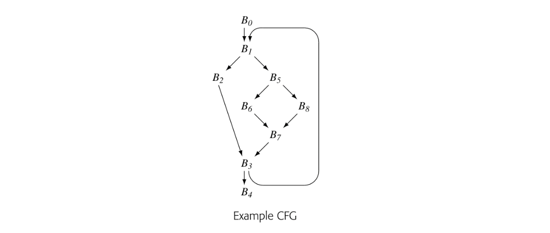
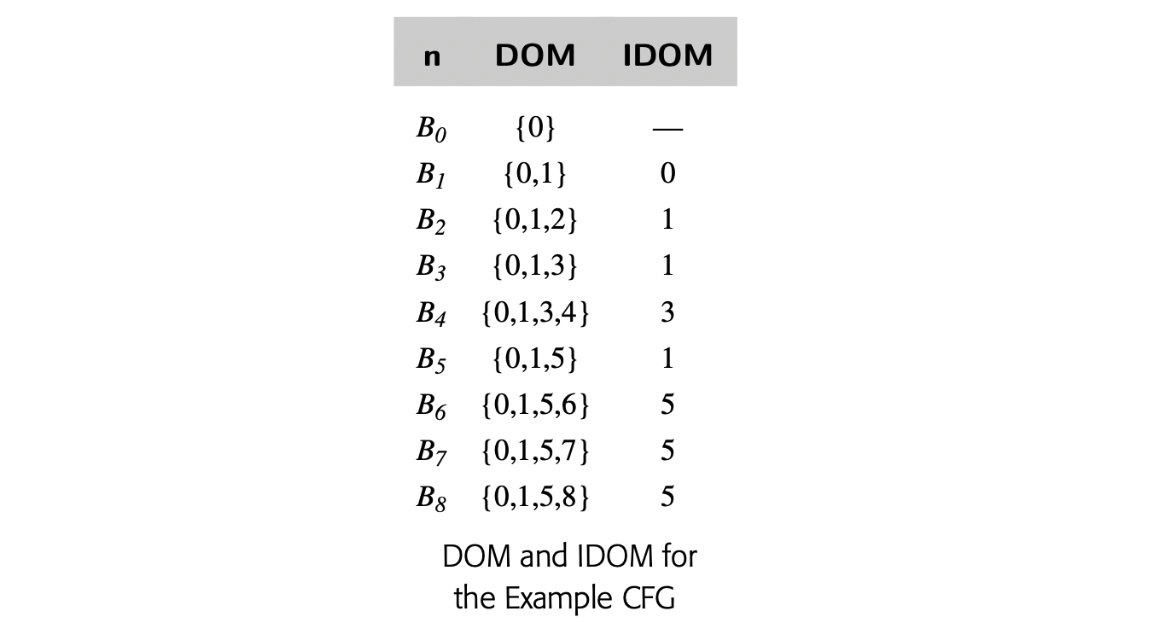
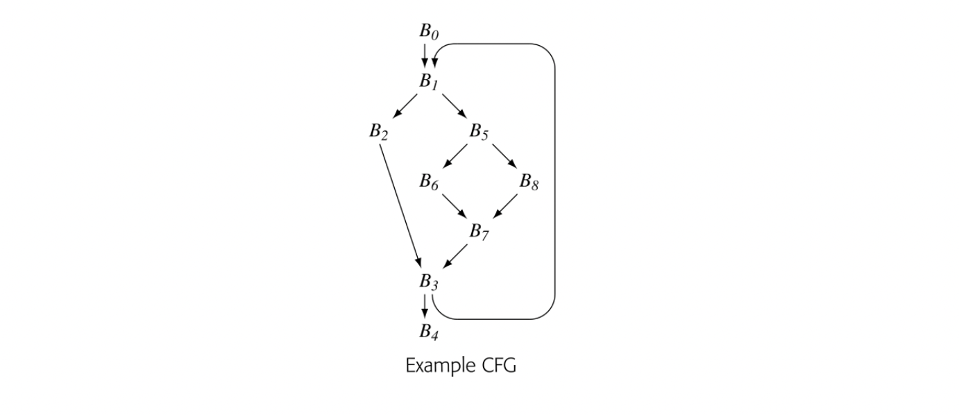
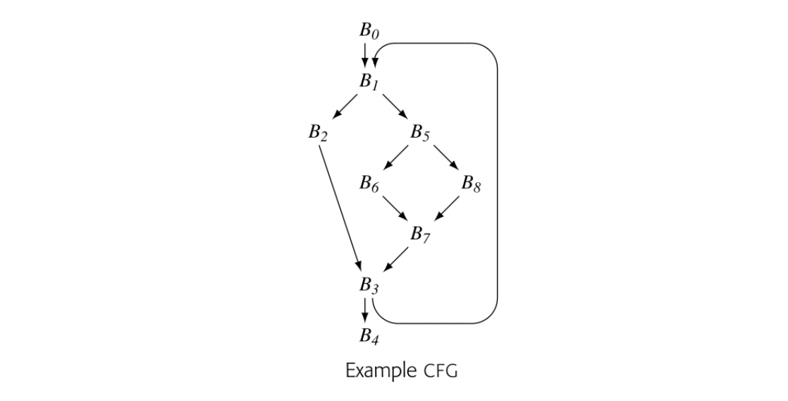
To make the notion of dominance concrete, consider node $B_6$ in the CFG shown in the margin. Every path from the entry node, $B_0$, to $B_6$ includes $B_0$, $B_1$, $B_5$, and $B_6$, so Dom($B_6$) is $\{B_0,B_1,B_5,B_6\}$. The table in the margin shows all of the Dom sets for the CFG.

For any CFG node $n$, one $m\in \text{DOM}(n)$, $m\ne n$, will be closer to $n$ in the CFG than any other $x\in \text{DOM}(n)$, $x\ne n$. That node, $m$, is the immediate dominator of $n$, denoted IDom($n$). By definition, a flow graph's entry node has no immediate dominator.

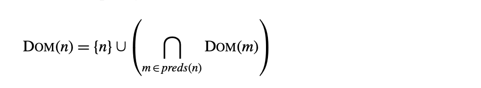
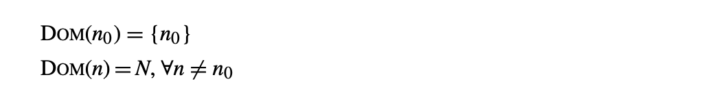
The following equations both define the Dom sets and form the basis of a method for computing them: To provide initial values, the compiler sets: where $N$ is the set of all nodes in the CFG. Given an arbitrary flow graph--that is, a directed graph with a single entry and a single exit--the equationsspecify the Dom set for each node. At each join point in the CFG, the equations compute the intersection of the Dom sets along each entering path. Because they specify Dom($n$) as a function of $n$'s predecessors, denoted $preds(n)$, information flows forward along edges in the CFG. Thus, the equations create a forward data-flow problem.

To solve the equations, the compiler can use the same three-step process used for live analysis in Section 8.6.1. It must (1) build a CFG, (2) gather initial information for each block, and (3) solve the equations to produce the Dom sets for each block. For Dom, step 2 is trivial; the computation only needs to know the node numbers.

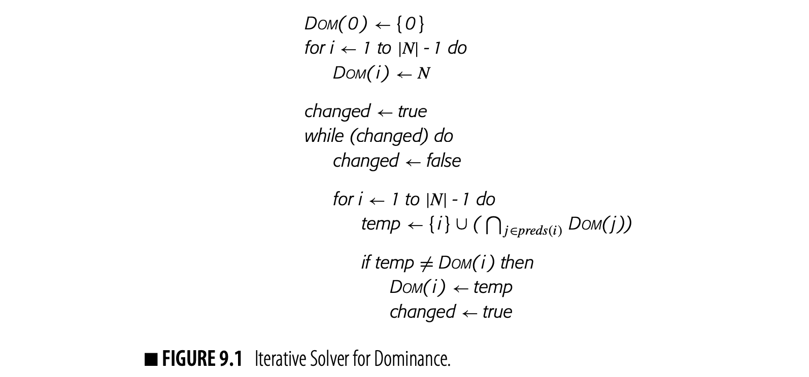
Fig. 9 shows a round-robin iterative solver for the dominance equations. It considers the nodes in order by their CFG name, $B_0$, $B_I$, $B_2$, and so on. It initializes the Dom set for each node, then repeatedly recomputes those Dom sets until they stop changing.

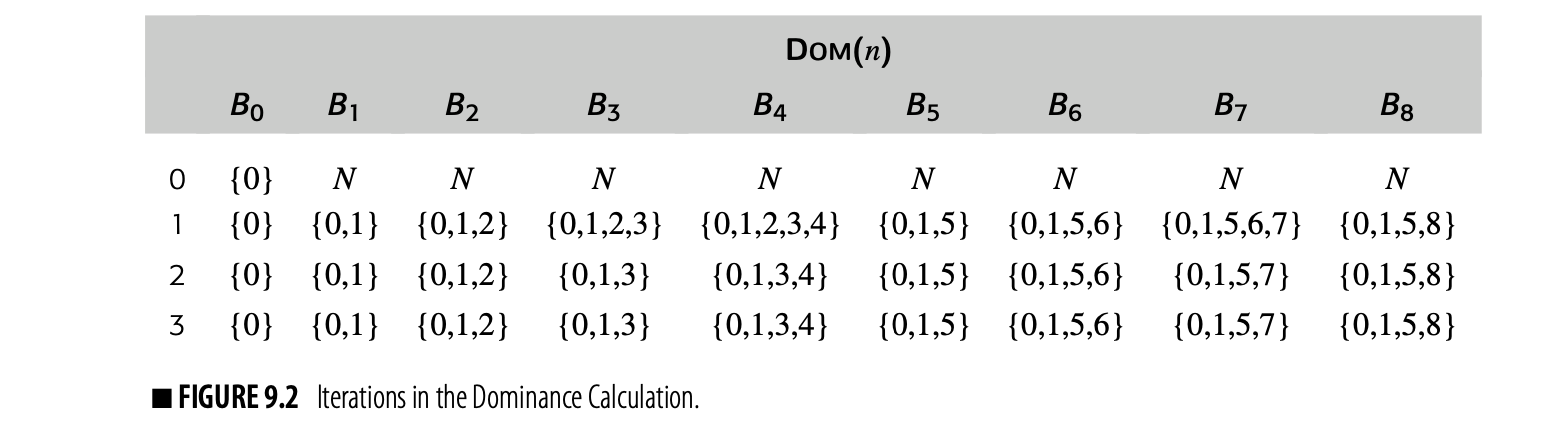
Fig. 2 shows how the values in the Dom sets change as the computation proceeds. The first column shows the iteration number; iteration zero shows the initial values. Iteration one computes correct Dom sets for any node with a single path from $B_0$, but computes overly large Dom sets for $B_3$, $B_4$, and $B_7$. In iteration two, the smaller Dom set for $B_7$ corrects the set for $B_3$, which, in turn shrinks Dom($B_4$). Similarly, the set for $B_8$ corrects the set for $B_7$. Iteration three shows that the algorithm has reached a fixed point.

Three critical questions arise regarding this solution procedure. First, does the algorithm halt? It iterates until the Dom sets stop changing, so the argument for termination is not obvious. Second, does it produce correct Dom sets? The answer is critical if we are to use Dom sets in optimizations. Finally, how fast is the solver? Compiler writers should avoid algorithms that are unnecessarily slow.

Termination

Iterative calculation of the Dom sets halts because the sets that approximate Dom shrink monotonically throughout the computation. The algorithm initializes Dom$(n_0)$ to $\{0\}$, and initializes the Dom sets for all other nodes to $N$, the set of all nodes. A Dom set can be no smaller than $\{0\}$ and can be no larger than $N$. Careful reasoning about the while loop shows that a Dom set, say Dom$(n_i)$, cannot grow from iteration to iteration. Either it shrinks, as the Dom set of one of its predecessors shrinks, or it remains unchanged.

The while loop halts when it makes a pass over the nodes in which no Dom set changes. Since the Dom sets can only change by shrinking and those sets are bounded in size, the while loop must eventually halt. When it halts, it has found a fixed point for this particular instance of the Dom computation.

Correctness

Recall the definition of dominance. Node $n_i$ dominates $n_j$ if and only if every path from the entry node $n_0$ to $n_j$ contains $n_i$. Dominance is a property of paths in the CFG.

Dom$(n_j)$ contains $i$ if and only if $i\in \text{Dom}(n_k)$ for all $k\in \text{preds}(j)$, or if $i=j$. The algorithm computes Dom$(n_j)$ as $j$ plus the intersection of the Dom sets of all $n_j$'s predecessors. How does this local computation over individual edges relate to the dominance property, which is defined over all paths through the CFG?

Meet operator In the theory of data-flow analysis, the meet $operator(\wedge )$ is used to combine facts at a join point in the CFG. In the $DOM$ equations, the meet operator is set intersection.

The Dom sets computed by the iterative algorithm form a fixed-point solution to the equations for dominance. The theory of iterative data-flow analysis, which is beyond the scope of this text, assures us that a fixed point exists for these particular equations and that the fixed point is unique [221]. This "all-paths" formulation of Dom describes a fixed-point for the equations, called the meet-over-all-paths solution. Uniqueness guarantees that the fixed point found by the iterative algorithm is identical to the meet-over-all-paths solution.

Efficiency

Postorder number a labeling of the graph’s nodes that corre- sponds to the order in which a postorder traversal would visit them

Because the fixed-point solution to the Dom equations for a specific CFG is unique, the solution is independent of the order in which the solver computes those sets. Thus, the compiler writer is free to choose an order of evaluation that improves the analyzer's running time.

The compiler can compute RPO numbers in a postorder traversal if it starts a counter at $|N|-1$ and decrements the counter as it visits and labels each node.

A $\text{reverse postorder}$ (RPO) traversal of the graph is particularly effective for forward data-flow problems. If we assume that the postorder numbers run from zero to $|N|$ - 1, then a node's rpo number is simply $|N|$ - 1 minus that node's postorder number. Here, $N$ is the set of nodes in the graph.

An RPO traversal visits as many of a node's predecessors as possible, in a consistent order, before visiting the node. (In a cyclic graph, a node's predecessor may also be its descendant.) A postorder traversal has the opposite property; for a node $n$, it visits as many of $n$'s successors as possible before visiting $n$. Most interesting graphs will have multiple rpo numberings; from the perspective of the iterative algorithm, they are equivalent.

For a forward data-flow problem, such as Dom, the iterative algorithm should use an rpo computed on the CFG. For a backward data-flow problem, such as LiveOut, the algorithm should use an rpo computed on the reverse cfg; that is, the cfg with its edges reversed. (The compiler may need to add a unique exit node to ensure that the reverse cfg has a unique entry node.)

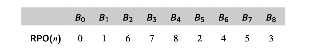
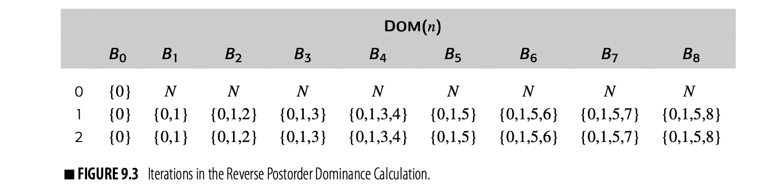
To see the impact of ordering, consider the impact of an rpo traversal on our example Dom computation. One rpo numbering for the example cfg, repeated in the margin, is:

Visiting the nodes in this order produces the sequence of iterations and val- ues shown in Fig. 9.3. Working in RPO, the algorithm computes accurate DOM sets for this graph on the first iteration and halts after the second iter- ation. RPO lets the algorithm halt in two passes over the graph rather than three. Note, however, that the algorithm does not always compute accurate DOM sets in the first pass, as the next example shows.

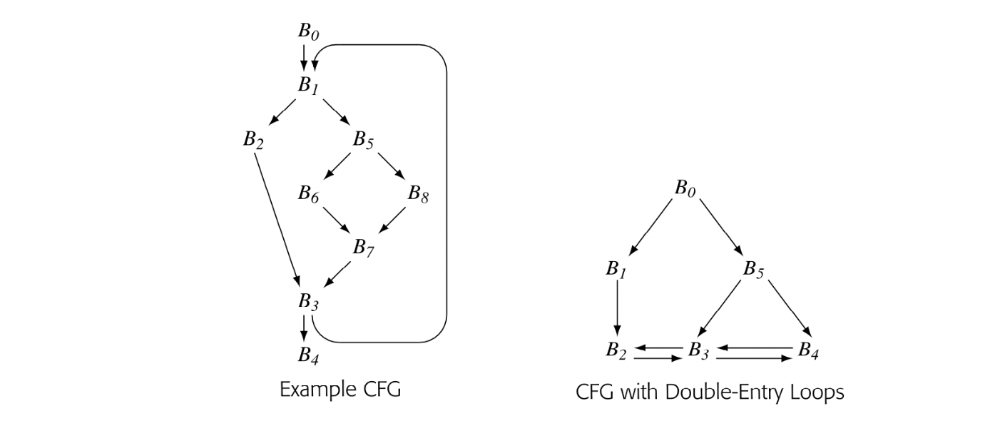
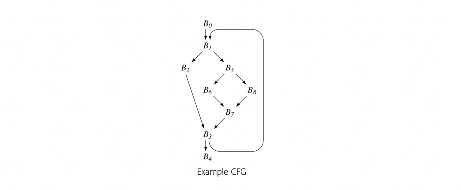
As a second example, consider the second CFG in the margin. It has two loops with multiple entries: $\left(B_2,B_3\right)$ and $\left(B_3,B_4\right)$. In particular,$\left(B_2,B_3\right)$ has entries from both $\left(B_0,B_1,B_2\right)$ and $\left(B_0,B_5,B_3\right)$, while $\left(B_3,B_4\right)$ has entries

from $(B_0,B_5,B_3)$ and $(B_0,B_5,B_4)$. This property makes the graph irreducible, which makes it more difficult to analyze with some data-flow algorithms (see the discussion of reducibility in Section 9.5.1).

To apply the iterative algorithm, we need an rpo numbering. One rpo numbering for this CFG is: Working in this order, the algorithm produces the following iterations:

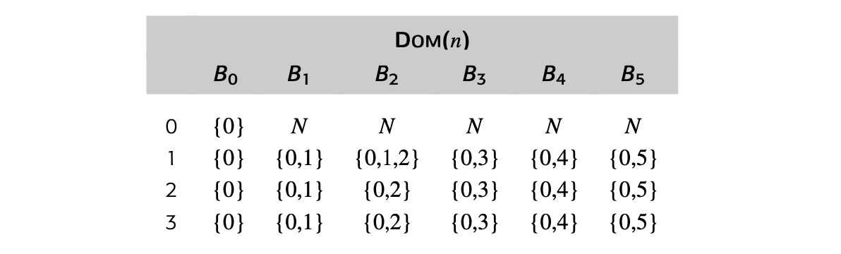
The algorithm requires two iterations to compute the correct DOM sets. The final iteration recognizes that it has reached a fixed point.

The dominance calculation relies only on the structure of the graph. It ig- nores the behavior of the code in any of the CFG’s blocks. As such, it might be considered a form of control-flow analysis. Most data-flow problems in- volve reasoning about the behavior of the code and the flow of data between operations. As an example of this kind of calculation, we will revisit the analysis of live variables.

9.2.2 Live-VariableAnalysis

NAMING SETS IN DATA-FLOW EQUATIONS

In writing the data-flow equations for classic problems, we have renamed the sets that contain local information. The original papers use more intuitive set names. Unfortunately, those names clash with each other across problems. For example, available expressions, live variables, reaching definitions, and anticipable expressions all use some notion of a kill set. These four problems, however, are defined over three distinct domains: expressions (AVAILOUT and ANTOUT), definition points (REACHES), and variables (LIVEOUT). Thus, using one set name, such as KILL or KILLED, can produce confusion across problems.

The names that we have adopted encode both the domain and a hint as to the set’s meaning. Thus, VARKILL(n) contains the set of variables killed in block n, while EXPRKILL(n) contains the set of expressions killed in the same block. Similarly, UEVAR(n) is the set of upward-exposed variables in n, while UEEXPR(n) is the set of upward-exposed expressions. While these names are somewhat awkward, they make explicit the distinction between the notion of kill used in available expressions (EXPRKILL) and the one used in reaching definitions (DEFKILL).

In Section 8.6.1, we used the results of live analysis to identify uninitialized variables. Compilers use live information for many other purposes, such as register allocation and construction of some variants of SSA form. We formulated live analysis as a global data-flow problem with the equation:

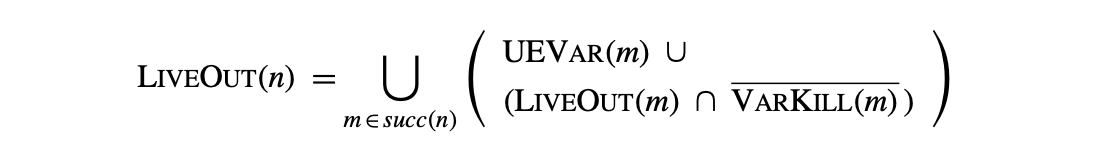
where, succ(n) refers to the set of CFG successors of $n$. The analysis should initialize $\text{LiveOut}(n)=\varnothing ,\forall n$.

Comparing the equations for LiveOut and Dom reveals differences between the problems.

• LiveOut is a backward data-flow problem; $\text{LiveOut}(n)$ is a function of the information known on entry to each of $n$'s CFG successors. By contrast, Dom is a forward data-flow problem.
• LiveOut looks for a future use on any path in the CFG; thus, it combines information from multiple paths with the union operator. Dom looks for predecessors that lie on all paths from the entry node; thus, it combines information from multiple paths with the intersection operator.
• LiveOut reasons about the effects of operations. The sets $\text{UEVAR}(n)$ and $\text{VarKill}(n)$ encode the effects of executing the block associated with $n$. By contrast, the Dom equations only use node names. LiveOut uses more information and takes more space.

Despite the differences, the process for solving an instance of LiveOut is the same as for an instance of Dom. The compiler must: (1) build a CFG; (2) compute initial values for the sets (see Fig. 8.15(a) on page 420), and (3) apply the iterative algorithm (see Fig. 8.15(b)). These steps are analogous to those taken to solve the Dom equations.

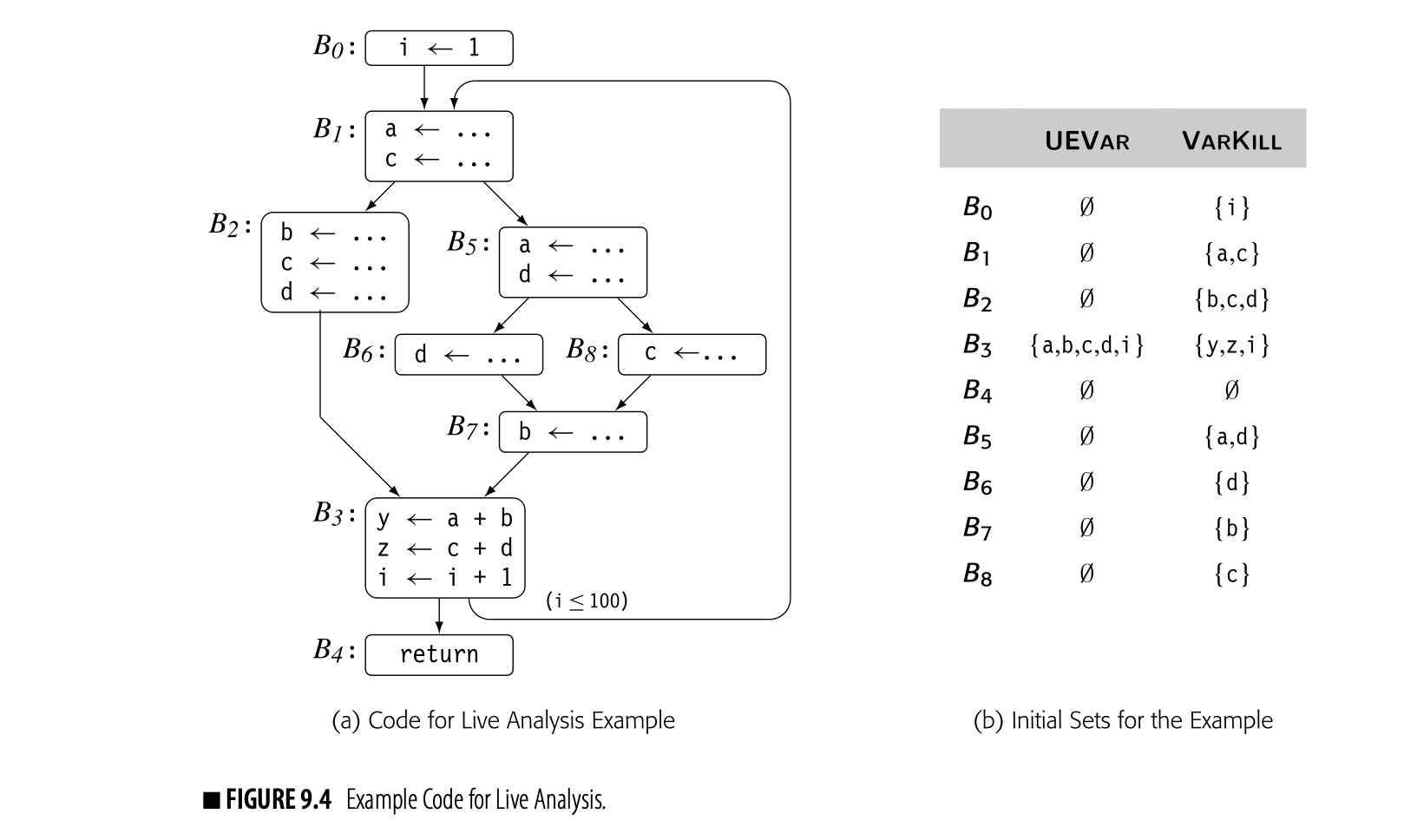
To see the issues that arise in solving an instance of LiveOut, consider the code shown in Fig. 9.4(a). It fleshes out the example CFG that we have used throughout this chapter. Panel (b) shows the UEVar and VarKill sets for each block.

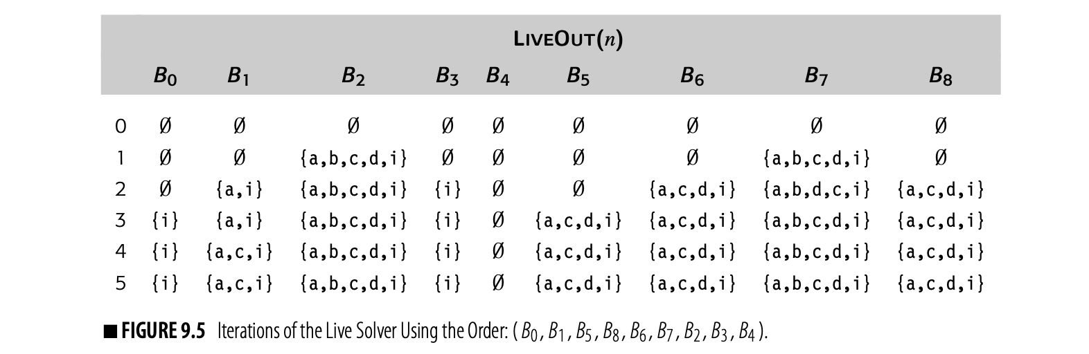
Fig. 9.5 shows the progress of the iterative solver on the example from Fig. 9.4(a), using the same RPO that we used in the Dom computation. Although the equations for LiveOut are more complex than those for Dom, the arguments for termination, correctness, and efficiency are similar to those for the dominance equations.

Termination

Recall that in DOM the sets shrink monoton- ically.

Iterative live analysis halts because the sets grow monotonically and the sets have a finite maximum size. Each time that the algorithm evaluates the LiveOut equation at a node in the cfg, that LiveOut set either remains the same or it grows larger. The LiveOut sets do not shrink. When the algorithm reaches a state where no LiveOut set changes, it halts. It has reached a fixed point.

The LiveOut sets are finite. Each LiveOut set is either $V$, the set of names being analyzed, or it is a proper subset of $V$. In the worst case, one LiveOut set would grow by a single name in each iteration; that behavior would halt after $n\cdot |V|$ iterations, where $n$ is the number of nodes in the cfg.

This property-the combination of monotonicity and finite sets-guarantees termination. It is often called the finite descending chain property. In Dom, the sets shrink monotonically and their size is less than or equal to the number of nodes in the cfg. In LiveOut, the sets grow monotonically and their size is bounded by the number of names being analyzed. Either way, it guarantees termination.

Correctness

Iterative live analysis is correct if and only if it finds all the variables that satisfy the definition of liveness at the end of each block. Recall the definition: A variable $v$ is live at point $p$ if and only if there is a path from $p$ to a use of $v$ along which $v$ is not redefined. Thus, liveness is defined in terms of paths in the cfg. A path that contains no definitions of $v$ must exist from $p$ to a use of $v$. We call such a path a $v$-clear path.

$\text{LiveOut}(n)$ should contain $v$ if and only if $v$ is live at the end of block $n$. To form $\text{LiveOut}(n)$, the iterative solver computes the contribution to $\text{LiveOut}(n)$ of each successor of $n$ in the cfg. The contribution of some successor $m$ to $\text{LiveOut}(n)$ is given by the right-hand side of the $\text{LiveOut}$ equation: $\text{UEVar}(m)$$\cup$ ($\text{LiveOut}(m)\cap \overline{\text{VarKill}(m)}$).

The solver combines the contributions of the various successors with union because $v\in \text{LiveOut}(n)$ if $v$ is live on any path that leaves $n$.

How does this local computation over single edges relate to liveness defined over all paths? The LiveOut sets that the solver computes are a fixed-point solution to the live equations. Again, the theory of iterative data-flow analysis assures us that the live equations have a unique fixed-point solution [221]. Uniqueness guarantees that all the fixed-point solutions are identical, which includes the meet-over-all-paths solution implied by the definition.

Efficiency

It is tempting to think that reverse postorder on the reverse CFG is equivalent to reverse preorder on the CFG. Exercise 3.b shows a counter-example.

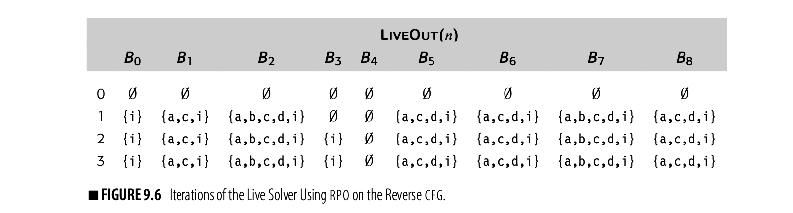
For a backward problem, the solver should use an rpo traversal on the reverse cfg. The iterative evaluation shown in Fig. 9.5 used rpo on the cfg. For the example cfg, one rpo on the reverse cfg is:

Visiting the nodes in this order produces the iterations shown in Fig. 9.6. Now, the algorithm halts in three iterations, rather than the five iterations required with a traversal ordered by rpo on the cfg. Comparing this table against the earlier computation, we can see why. On the first iteration, the algorithm computed correct LiveOut sets for all nodes except $B_3$. It took a second iteration for $B_3$ because of the back edge--the edge from $B_3$ to $B_1$. The third iteration is needed to recognize that the algorithm has reached its fixed point. Since the fixed point is unique, the compiler can use this more efficient order.

This pattern holds across many data-flow problems. The first iteration computes sets that are correct, except for the effects of cycles. Subsequent iterations settle out the information from cycles.

9.2.3 Limitations on Data-Flow Analysis

There are limits to what a compiler can learn from data-flow analysis. In some cases, the limits arise from the assumptions underlying the analysis. In other cases, the limits arise from features of the language being analyzed. To make informed decisions, the compiler writer must understand what data-flow analysis can do and what it cannot do.

When it computes $\text{LiveOut}(n)$, the iterative algorithm uses the sets $\text{LiveOut}$, $\text{UEVar}$, and $\text{VarKill}$ for each of $n$'s CFG successors. This action implicitly assumes that execution can reach each of those successors; in practice, one or more of them may not be reachable.

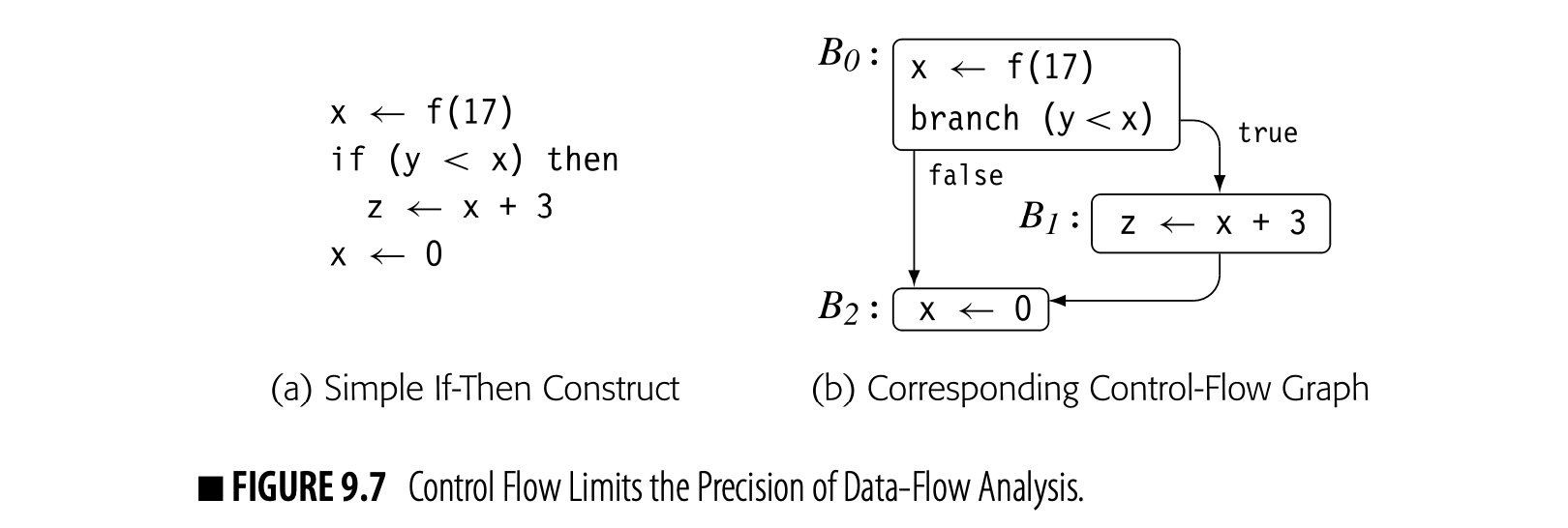
Consider the code fragment shown in Fig. 9.7 along with its CFG. The definition of x in $B_O$ is live on exit from $B_O$ because of the use of x in $B_I$. The definition of x in $B_2$ kills the value set in $B_O$. If $B_I$ cannot execute, then x's value from $B_O$ is not live past the comparison with y, and x # $\text{LiveOut}(B_O)$. If the compiler can prove that the y is always less than x, then $B_I$ never executes. The compiler can eliminate $B_I$ and replace the test and branch in $B_O$ with a jump to $B_2$. At that point, if the call to f has no side effects, the compiler can also eliminate $B_O$.

The equations for $\text{LiveOut}$, however, take the union over all successors of a block, not just its executable successors. Thus, the analyzer computes:

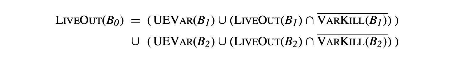
Data-flow analysis assumes that all paths through the CFG are feasible. Thus, the information that they compute summarizes the possible data-flow events, assuming that each path can be taken. This limits the precision of the resulting information; we say that the information is precise "up to symbolic execution." With this assumption, x $\in \text{LiveOut}(B_O)$ and both $B_O$ and $B_I$ must be preserved.

STATIC ANALYSIS VERSUS DYNAMIC ANALYSIS

The notion of static analysis leads directly to the question: What about dynamic analysis? By definition, static analysis tries to estimate, at compile time, what will happen at runtime. In many situations, the compiler cannot tell what will happen, even though the answer might be obvious with knowledge of one or more runtime values.

Consider, for example, the C fragment:

It contains a redundant expression, $y\ast z$, if and only if p does not contain the address of either y or z. At compile time, the value of p and the address of y and z may be unknown. At runtime, they are known and can be tested. Testing these values at runtime would allow the code to avoid recomputing $y\ast z$, where compile-time analysis might be unable to answer the question.

However, the cost of testing whether $p==\&y$, or $p==\&z$, or neither and acting on the result is likely to exceed the cost of recomputing y * z. For dynamic analysis to make sense, it must be a priori profitable—that is, the savings must exceed the cost of the analysis. This happens in some cases; in most cases, it does not. By contrast, the cost of static analysis can be amortized over multiple executions of the code, so it is more attractive, in general.

Another way that imprecision creeps into the results of data-flow analysis comes from the treatment of arrays, pointers, and procedure calls. An array reference, such as A[i,j], refers to a single element of A. However, without analysis that reveals the values of i and j, the compiler cannot tell which element of A is accessed. For this reason, compilers have traditionally treated a reference to an element of A as a reference to all of A. Thus, a use of A[i,j] counts as a use of A, and a definition of A[m,n] counts as a definition of A.

The compiler writer must not, however, make too strong an inference. Because the information on arrays is imprecise, the compiler must interpret that information conservatively. Thus, if the goal of the analysis is to determine where a value is no longer live--that is, the value must have been killed--then a definition of A[i,j] does not kill the value of A. If the goal is to recognize where a value might not survive, then a definition of A[i,j] might define any element of A.

Points-to analysis, used to track possible pointer values, is more expensive than classic data-flow problems such as DOM and LIVE.

Pointers add another level of imprecision to the results of static analysis. Explicit arithmetic on pointers makes matters worse. Unless the compiler employs an analysis that tracks the values of pointers, it must interpret an assignment to a pointer-based variable as a potential definition for every variable that the pointer might reach. Type safety can limit the set of objects that the pointer can define; a pointer declared to point at an object of type $t$ can only be used to modify objects of type $t$. Without analysis of pointer values or a guarantee of type safety, assignment to a pointer-based variable can force the analyzer to assume that every variable has been modified. In practice, this effect often prevents the compiler from keeping the value of a pointer-based variable in a register across any pointer-based assignment. Unless the compiler can specifically prove that the pointer used in the assignment cannot refer to the memory location corresponding to the enregistered value, it cannot safely keep the value in a register.

The complexity of analyzing pointer use leads many compilers to avoid keeping values in registers if they can be the target of a pointer. Usually, some variables can be exempted from this treatment--such as a local variable whose address has never been explicitly taken. The alternative is to perform data-flow analysis aimed at disambiguating pointer-based references--reducing the set of possible variables that a pointer might reference at each point in the code. If the program can pass pointers as parameters or use them as global variables, pointer disambiguation becomes inherently interprocedural.

Procedure calls provide a final source of imprecision. To understand the data flow in the current procedure, the compiler must know what the callee can do to each variable that is accessible to both the caller and the callee. The callee may, in turn, call other procedures that have their own potential side effects.

Unless the compiler computes accurate summary information for each procedure call, it must estimate the call's worst-case behavior. While the specific assumptions vary across problems and languages, the general rule is to assume that the callee both uses and modifies every variable that it can reach. Since few procedures modify and use every variable, this rule typically overestimates the impact of a call, which introduces further imprecision into the results of the analysis.

9.2.4 Other Data-Flow Problems

Compilers use data-flow analyses to prove the safety of applying transformations in specific situations. Thus, many distinct data-flow problems have been proposed, each for a particular optimization.

Availability

Availability An expression $e$ is available at point $p$ if and only if, on every path from the procedure's entry to $p$, $e$ is evaluated and none of its operands is redefined.

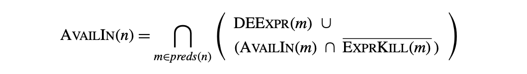
To identify redundant expressions, the compiler can compute information about the availability of expressions. This analysis annotates each node $n$ in the CFG with a set $\text{AvailIn}(n)$, which contains the names of all expressions in the procedure that are available on entry to the block corresponding to $n$. The equations for $\text{AvailIn}$ are:

with initial values for the $\text{AvailIn}$ sets:

These equations can be solved efficiently with a standard iterative data-flow solver. Since it is a forward data-flow problem, the solver should use RPO on the CFG.

In the equations, $\text{DEExpr}(n)$ is the set of downward-exposed expressions in $n$. An expression $e\in \text{DEExpr}(n)$ if and only if block $n$ evaluates $e$ and none of $e$'s operands is defined between the last evaluation of $e$ in $n$ and the end of $n$. $\text{ExprKill}(n)$ contains all those expressions that are killed by a definition in $n$. An expression is killed if one or more of its operands are redefined in the block.

An expression $e$ is available on entry to $n$ if and only if it is available on exit from each of $n$'s predecessors in the CFG. As the equation states, an expression $e$ is available on exit from some block $m$ if one of two conditions holds: either $e$ is downward exposed in $m$, or it is available on entry to $m$ and is not killed in $m$.

AvailIn sets are used in global redundancy elimination, sometimes called global common subexpression elimination. Perhaps the simplest way to achieve this effect is to compute $\text{AvailIn}$ sets for each block and use them as initial information in local value numbering (see Section 46.1). Lazy code motion is a stronger form of redundancy elimination that also uses availability (see Section 46.1).

Reaching Definitions

In some cases, the compiler needs to know where an operand was defined. If multiple paths in the CFG lead to the operation, then multiple definitions may provide the value of the operand. To find the set of definitions that reacha block, the compiler can compute reaching definitions. The compiler annotates each node $n$ in the CFG with a set, $\text{Reaches}(n)$ that contains the name of every definition that reaches the head of the block corresponding to $n$. The domain of $\text{Reaches}$ is the set of definition points in the procedure--the set of assignments.

The compiler computes a set $\text{Reaches}(n)$ for each CFG node $n$ using the equation:

with initial values for the Reaches sets: $\text{DEDef}(m)$ is the set of downward-exposed definitions in $m$: those definitions in $m$ for which the defined name is not subsequently redefined in $m$. $\text{DefKill}(m)$ contains all the definition points that are obscured by a definition of the same name in $m$; $d\in \text{DefKill}(m)$ if $d$ defines some name $v$ and $m$ contains a definition that also defines $v$. Thus, $\overline{\text{DefKill}(m)}$ contains those definition points that survive through $m$.

$\text{DEDef}$ and $\text{DefKill}$ are both defined over the set of definition points, but computing each of them requires a mapping from names (variables and compiler-generated temporaries) to definition points. Thus, gathering the initial information for reaching definitions is more expensive than it is for live variables.

Anticipable Expressions

Anticipability An expression, $e$, is anticipable at point $p$ if and only if (1) every path that leaves $p$ evaluates $e$, and (2) evaluating $e$ at $p$ would produce the same result as the first evaluation along each of those paths.

In some situations, the compiler can move an expression backward in the CFG and replace multiple instances of the $expression$, along different paths, with a single instance. This optimization, called hoisting, reduces code size. It does not change the number of times the expression is evaluated.

To find safe opportunities for hoisting, the compiler can compute the set of anticipable expressions at the end of each block. An expression $e$ is anticipable at the end of block $b$ if the next evaluation of $e$, along each path leaving $b$, would produce the same result. The equations require that $e$ be computed along every path that leaves $b$.

$\text{AntOut}$, the set of expressions anticipable at the end of a block, can be computed as a backward data-flow problem on the CFG. Anticipability is formulated over the domain of expressions.

Implementing Data-Flow Frameworks

The equations for many global data-flow problems show a striking similarity. For example, available expressions, live variables, reaching definitions, and anticipable expressions all have propagation functions of the form: where $c_1$ and $c_2$ are constants derived from the code and $o{p}_1$ and $o{p}_2$ are standard set operations such as $\cup$ and $\cap$. This similarity appears in the problem descriptions; it creates the opportunity for code sharing in the implementation of the analyzer.

The compiler writer can easily abstract away the details in which these problems differ and implement a single, parameterized analyzer. The analyzer needs functions to compute $c_1$ and $c_2$, implementations of the operators, and an indication of the problem's direction. In return, it produces the desired data-flow sets.

This implementation strategy encourages code reuse. It hides the low-level details of the solver. It also creates a situation in which the compiler writer can profitably invest effort in optimizing the implementation. For example, a scheme that implements $f(x)=c_{1}o{p}_1(xo{p}_2{c}_2)$ as a single function may outperform one that implements both $f_1(x)=c_{1}o{p}_{1}x$ and $f_2(x)=xo{p}_2{c}_2$, and computes $f(x)$ as $f_1(f_2(x))$. A framework lets all the client transformations benefit from improvements in the set representations and operator implementations.

The equations to define AntOut are:

with initial values for the AntOut sets:

Here $UEEXPR(m)$ is the set of upward-exposed expressions—those used in $m$ before they are killed. $EXPRKILL(m)$ contains all those expressions that are killed by a definition in $m$; it also appears in the equations for available expressions.

The results of anticipability analysis are used in lazy code motion, to de- crease execution time, and in code hoisting, to shrink the size of the compiled code. Both transformations are discussed in Section 10.3.

Interprocedural Summary Problems

When analyzing a single procedure, the compiler must account for the impact of each procedure call. In the absence of specific information about the call, the compiler must make worst-case assumptions about the callee and about any procedures that it, in turn, calls. These assumptions can seriously degrade the precision of the global data-flow information. For example, the compiler must assume that the callee modifies every variable that it can access; this assumption essentially stops the propagation of facts across a call site for all global variables, module-level variables, and call-by-reference parameters.

To limit such impact, the compiler can compute summary information on each call site. The classic summary problems compute the set of variables that might be modified as a result of the call and that might be used as a result of the call. The compiler can then use these computed summary sets in place of its worst case assumptions.

Flow insensitive This formulation of MAYMOD ignores control flow inside procedures. Such a formulation is said to be flow $insensitive$.

The $interprocedural$ may modify problem_ annotates each call site with a set of names that the callee, and procedures it calls, might modify. May modify is one of the simplest problems in interprocedural analysis, but it can have a significant impact on the quality of information produced by other analyses, such as global constant propagation. May modify is posed as a set of data-flow equations over the program's call graph that annotate each procedure with a MayMod set.

$MAYMOD(p)$ is initialized to contain all the names modified locally in $p$ that are visible outside $p$. It is computed as the set of names defined in $p$ minus any names that are strictly local to $p$.

The function $unbin{d}_e$ maps one set of names into another. For a call-graph edge $e=(p,q)$ and set of names $s$, $unbin{d}_e(s)$ maps each name in s from the name space of $q$ to the name space that holds at the call site, using the bindings at the call site that corresponds to $e$. In essence, it projects s from $q$ 's name space into p 's name space.

Given a set of $LOCALMOD$ sets and a call graph, an iterative solver will find a fixed-point solution for these equations. It will not achieve the kind of fast time bound seen in global data-flow analysis. A more complex framework is required to achieve near-linear complexity on this problem (see Chapter Notes).

The MayMod sets computed by these equations are generalized summary sets. That is, MayMod($q$) contains the names of variables that might be modified by a call to $q$, expressed in the name space of $q$. To use this information at a specific call site that invokes $q$, the compiler will compute the set $S={unbind}_e(\text{MayMod}(q))$, where $e=(p,q)$ is the call graph edge corresponding to the call. The compiler must then add to $S$ any names that are aliased inside $p$ to names contained in $S$.

The compiler can also compute the set of variables that might be referenced as a result of executing a procedure call, the interprocedural may reference problem. The equations to annotate each procedure $p$ with a set MayRef($p$) are similar to the equations for $MayMod$The function unbind e_{e} maps one set of names into another. For a call-graph edge e=(p, q) and set of names s, unbind d_{e}(s) maps each name in s from the name space of q to the name space that holds at the call site, using the bindings at the call site that corresponds to e. In essence, it projects s from q 's name space into p 's name space.\\Given a set of LOCALMOD sets and a call graph, an iterative solver will find a fixed-point solution for these equations. It will not achieve the kind of fast time bound seen in global data-flow analysis. A more complex framework is required to achieve near-linear complexity on this problem (see Chapter Notes)..

Section Review

Iterative data-flow analysis works by repeatedly reevaluating an equation at each node in some underlying graph until the sets defined by the equations reach a fixed point. Many data-flow problems have a unique fixed point, which ensures a correct solution independent of the evaluation order, and the finite descending chain property, which guarantees termination independent of the evaluation order. These two properties allow the compiler writer to choose evaluation orders that converge quickly. As a result, iterative analysis is robust and efficient.

The literature describes many different data-flow problems. Examples in this section include dominance, live analysis, availability, anticipability, and interprocedural summary problems. All of these, save for the interprocedural problems, have straightforward efficient solutions with the iterative algorithm. To avoid solving multiple problems, compilers often turn to a unifying framework, such as SSA form, described in the next section.

Review Questions

1. Compute Dom sets for the CFG shown in the margin, evaluating the nodes in the order $(B_d,B_2,B_1,B_5,B_3,B_0)$. Explain why this order takes a different number of iterations than is shown on page 456.
2. When the compiler builds a call graph, ambiguous calls can complicate the process, much as ambiguous jumps complicate CFG construction. What language features might lead to an ambiguous call site--one where the compiler was uncertain of the callee5 identify?

9.3 Static Single-Assignment Form

Over time, compiler writers have formulated many different data-flow problems. If each transformation uses its own analysis, the effort spent implementing, debugging, and maintaining the analysis passes can grow unreasonably large. To limit the number of analyses that the compiler writer must implement and that the compiler must run, it is desirable to use a single analysis for multiple transformations.

Some compilers, such as LLVM/CLANG, use SSA as their definitive IR.

One strategy for such a "universal" analysis is to build an IR called static single-assignment form (ssa) (see also Section 4.6.2). SSA encodes both data flow and control flow directly into the IR. Many of the classic scalar optimizations have been reworked to operate on code in SSA form.

Code in SSA form obeys two rules:

1. Each computation in the procedure defines a unique name.
2. Each use in the procedure refers to a single name.

The first rule removes the effect of "kills" from the code; any expression in the code is available at any point after it has been evaluated. (We first saw this effect in local value numbering.) The second rule has a more subtle effect. It ensures that the compiler can still represent the code concisely and correctly; a use can be written with a single name rather than a long list of all the definitions that might reach it. 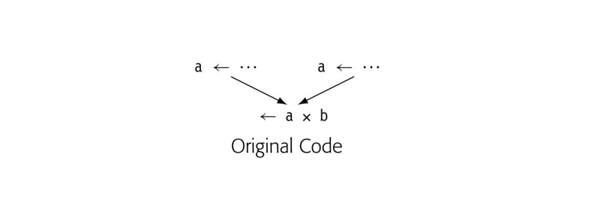Consider the small example shown in the margin. If the compiler renames the two definitions of a to a and, what name should appear in the use of a in a? Neither nor will work in a?b. (The example assumes that was defined earlier in the code.)

To manage this name space, the SSA construction inserts a special kind of copy operation, a $\varphi$-function, at the head of the block where control-flow paths meet, as shown in the margin. When the $\varphi$-function evaluates, it reads the argument that corresponds to the edge from which control flow entered the block. Thus, coming from the block on the left, the $\varphi$-function reads, while from the block on the right it reads. The selected argument is assigned to. Thus, the evaluation of computes the same value that did in the pre-SSA code.

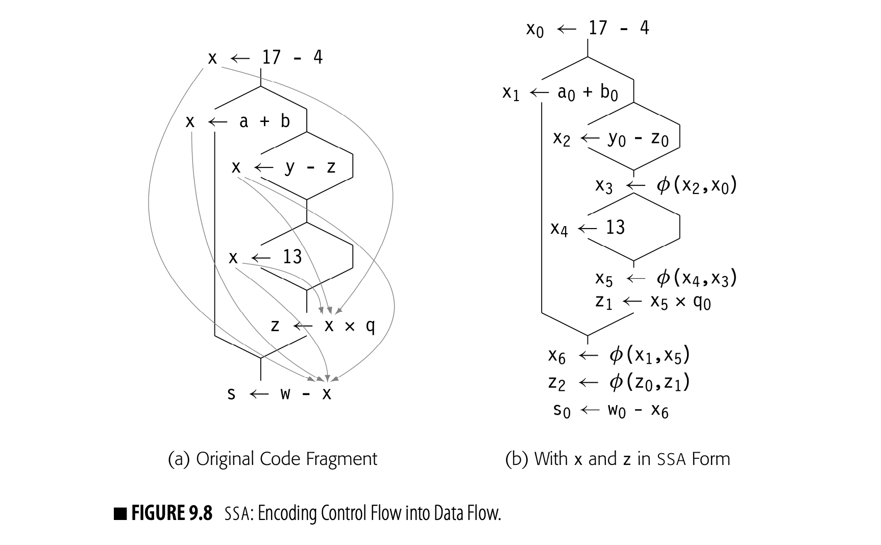Fig. 9.8 shows a more extensive example. Consider the various uses of the variable $x$ in the code fragment shown in panel (a). The curved gray lines show which definitions can reach each use of $x$. Panel (b) shows the same fragment in SSA form. Variables have been renamed with subscripts to ensure unique names for each definition. We assume that, and are defined earlier in the code.

The code in panel (b) includes all of the $\varphi$-functions needed to reconcile the names generated by rule one with the need for unique names in uses. Tracing the flow of values will reveal that the same values follow the same paths as in the original code.

Two final points about $\varphi$-functions need explanation. First, $\varphi$-functions are defined to execute concurrently. When control enters a block, all of the block's $\varphi$-functions read their designated argument, in parallel. Next, they all define their target names, in parallel. This concurrent execution semantics allows the SSA construction algorithm to ignore the order of $\varphi$-functions as it inserts them into a block.

Second, by convention, we write the arguments of a $\varphi$-function left-to-right to correspond with the incoming edges left-to-right on the printed page. Inside the compiler, the IR has no natural notion of left-to-right for the edges entering a block. Thus, the implementation will require some bookkeeping to track the correspondence between $\varphi$-function arguments and CFG edges.

9.3.1 A Naive Method for Building SSA Form

Both of the SSA-construction algorithms that we present follow the same basic outline: (1) insert $\varphi$-functions as needed and (2) rename variables and temporary values to conform with the two rules that define SSA form. The simplest construction method implements the two steps as follows:

The "naive" algorithm inserts more $\varphi$-functions than are needed. It adds a $\varphi$ - function for each name at each join point.

1. Inserting $\varphi$-functions At the start of each block that has multiple CFG predecessors, insert a $\varphi$-function, such as x $\leftarrow \varphi$(x,x), for each name x that the current procedure defines. The $\varphi$-function should have one argument for each predecessor block in the CFG. This process inserts a $\varphi$-function in every case that might need one. It also inserts many extraneous $\varphi$-functions.
2. Renaming The $\varphi$-function insertion algorithm ensures that a $\varphi$-function for $x$ is in place at each join point in the CFG reached by two or more definitions of $x$. The renaming algorithm rewrites all of the names into the appropriate SSA names. The first step adds a unique subscript to the name at each definition.

Base name In an SSA name $x_2$, the base name is x and the version is 2 .

At this point, each definition has a unique SSA name. The compiler can compute reaching definitions (see Section 9.2.4) to determine which SSA name reaches each use. The compiler writer must change the meaning of DefKill so that a definition to one SSA name kills not only that SSA name but also all SSA names with the same base name. The effect is to stop propagation of an SSA name at any $\varphi$-function where it is an argument. With this change, exactly one definition--one SSA name--reaches each use. The compiler makes a pass over the code to rewrite the name in each use with the SSA name that reaches it. This process rewrites all the uses, including those in $\varphi$-function arguments. If the same SSA name reaches a $\varphi$-function along multiple paths, the corresponding $\varphi$-function arguments will have the same SSA name. The compiler must sort out the correspondence between incoming edges in the CFG and $\varphi$-function arguments so that it can rename each argument with the correct SSA name. While conceptually simple, this task requires some bookkeeping.

A $\varphi$-function $x_j\leftarrow \varphi \left(x_i,x_i\right)$ is redundant. A $\varphi$-function whose value is not live is considered dead.

The naive algorithm constructs SSA form that obeys the two rules. Each definition assigns to a unique name; each reference uses the name of a distinct definition. While the algorithm builds correct SSA form, it can insert $\varphi$-functions that are redundant or dead. These extra $\varphi$-functions may be problematic. The compiler wastes memory representing them and time traversing them. They can also decrease the precision of some kinds of analysis over SSA form.

We call this flavor of SSA maximal SSA form. To build SSA form with fewer $\varphi$-functions requires more work; in particular, the compiler must analyze the code to determine where potentially distinct values converge in the CFG. This computation relies on the dominance information described in Section 9.2.1.

The difference of SSA form of SSA Form

The literature proposes several distinct flavors of SSA form. The flavors differ in their criteria for inserting $\varphi$-functions. For a given program, they can produce different sets of $\varphi$-functions.

Minimal SSA inserts a $\varphi$-function at any join point where two distinct definitions for the same original name meet. This is the minimal number consistent with the definition of SSA. Some of those $\varphi$-functions, however, may be dead; the definition says nothing about the values being live when they meet.

Pruned SSA adds a liveness test to the $\varphi$-insertion algorithm to avoid adding dead $\varphi$-functions. The construction must compute LwEOUT sets, which increases the cost of building pruned SSA.

Semipruned SSA is a compromise between minimal SSA and pruned SSA. Before inserting $\varphi$-functions, the algorithm eliminates any names that are not live across a block boundary. This can shrink the name space and reduce the number of $\varphi$-functions without the overhead of computing LwEOUT sets. The algorithm in Fig. 9.11 computes semipruned SSA.

Of course, the number of $\varphi$-functions depends on the specific program being converted into SSA form. For some programs, the reductions obtained by semipruned SSA and pruned SSA are significant. Shrinking the SSA form can lead to faster compilation, since passes that use SSA form then operate on programs that contain fewer operations--and fewer $\varphi$-functions.

The following subsections present, in detail, an algorithm to build semipruned SSA--a version with fewer $\varphi$-functions. Section 9.3.2 introduces dominance frontiers and shows how to compute them; dominance frontiers guide $\varphi$-function insertion. Section 9.3.3 gives an algorithm to insert $\varphi$-functions, and Section 9.3.4 presents an efficient algorithm for renaming. Section 9.3.5 discusses complications that can arise in translating out of SSA form.

9.3.2 Dominance Frontiers

The primary problem with maximal SSA form is that it contains too many $\varphi$-functions. To reduce their number, the compiler must determine more carefully where they are needed. The key to $\varphi$-function insertion lies in understanding which names need a $\varphi$-function at each join point. To solve this problem efficiently and effectively, the compiler can turn the question around. It can determine, for each block $i$, the set of blocks that will need a $\varphi$-function as the result of a definition in block $i$. Dominance plays a critical role in this computation.

Consider the CFG shown in the margin. Assume that the code assigns distinct values to $a$ in both $B_I$ and $B_5$, and that no other block assigns to $a$. The value from $B_5$ is the only value for $a$ that can reach $B_6$, $B_7$, and $B_8$. Because $B_5$ dominates these three blocks, it lies on any path from $B_0$ to $B_6$, $B_7$, or $B_8$. The definition in $B_I$ cannot reach them.

Strict dominance In a CFG, node $p$ strictly dominates node $q$ if $p\in \mathrm{Dom}(q)$ and $p\ne q$. We denote this as $p\in (\mathrm{Dom}(q)-q)$.

$B_3$ presents a different situation. Neither of its CFG predecessors, $B_2$ and $B_7$, dominate $B_3$. A use of $a$ in $B_3$ can receive its value from either $B_I$ or $B_5$, depending on the path taken to reach $B_3$. The assignments to $a$ in $B_I$ and $B_5$ force a $\varphi$-function for $a$ at the start of $B_3$.

$B_5$ dominates the region $(B_6,B_7,B_8)$. It is the immediate dominator of all three nodes. A definition of $a$ in $B_5$ will reach a use in that region, unless $a$ is redefined before the use. The definition in $B_5$ cannot necessitate the need for a $\varphi$-function in this region.

Strict dominance In a CFG, node p strictly dominates node q if $p\in \mathrm{Dom}(q)$ and $p\ne q$. We denote this as $p\in (\mathrm{Dom}(q)-q)$.

$B_3$ lies just outside of the region that $B_5$ dominates. It has two CFG predecessors and $B_5$ only dominates one of them. Thus, it lies one CFG edge outside the region that $B_5$ dominates. In general, a definition of $a$ in some block $B_i$ will necessitate a $\varphi$-function in any node that, like $B_3$, lies one CFG edge beyond the region that $B_i$ dominates. The dominance frontier of $B_i$, denoted DF($B_i$), is the set of all such nodes.

Dominance frontier In a CFG, node $q$ is in the dominance frontier of node p if and only if (1) p dominates a CFG predecessor of $q$ and (2) p does not strictly dominate $q$. We denote p 's dominance frontier as $\mathrm{DF}(p)$.

To recap, $q\in$ DF($p$) if, along some path, $q$ is one edge beyond the region that $p$ dominates. Thus:

• $q$ has a CFG predecessor that $p$ dominates. There exists an $x$ such that $(x,q)$ is a CFG edge and $p\in \text{Dom}(x)$.
• $p$ does not strictly dominate $q$. That is, $p\notin (\text{Dom}(q)-q)$.

DF($p$) is simply the set of all nodes that meet these two criteria.

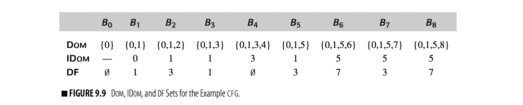
A definition of $a$ in block $n$ forces the insertion of a $\varphi$-function for $a$ at the head of each block $m\in$ DF($n$). Fig. 9 shows the Dom, IDom, and DF sets for the example CFG.

Notice the role of strict dominance. In the example CFG, strict dominance ensures that $B_1\in$ DF($B_1$). Thus, an assignment to some name $a$ in $B_1$ forces

the insertion of a $\varphi$-function in $B_1$. If the definition of dominance frontiers used Dom, instead, $\text{DF}(B_1)$ would be empty.

Dominator Trees

Dominator tree a tree that encodes the dominance informa- tion for a flow graph

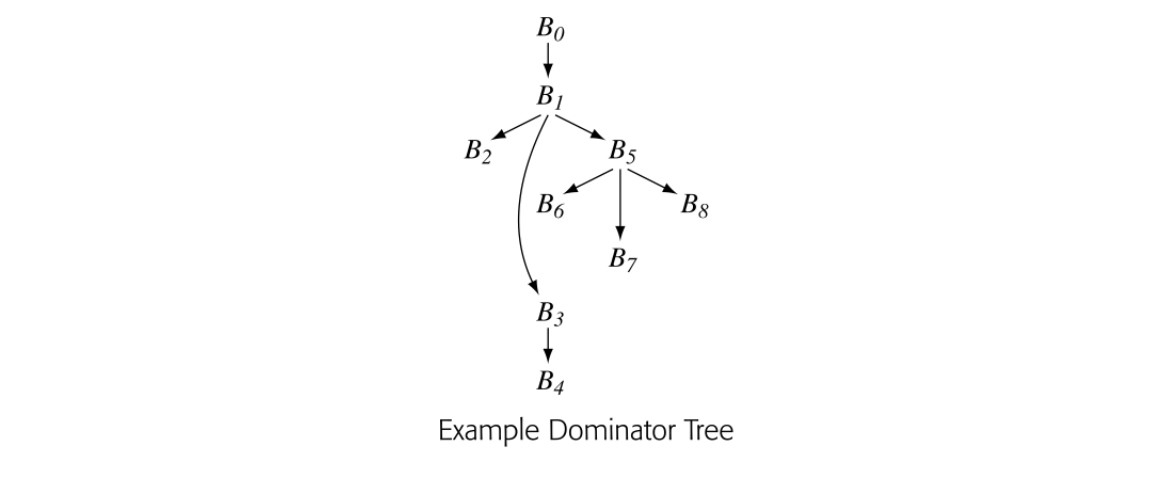
The algorithm to compute dominance frontiers uses a data structure, the dominator tree, to encode dominance relationships. The dominator tree of a CFG has a node for each block in the CFG. Edges encode immediate dominance; if $m=\text{IDom}(n)$, then $n$ is a child of $m$ in the dominator tree.

The dominator tree encodes the Dom sets as well. For a node $n$, $\text{Dom}(n)$ contains precisely the nodes on the path from $n$ to the root of the dominator tree. The nodes on that path are ordered by the IDom relationship. The dominator tree for our running example appears in the margin.

Computing Dominance Frontiers

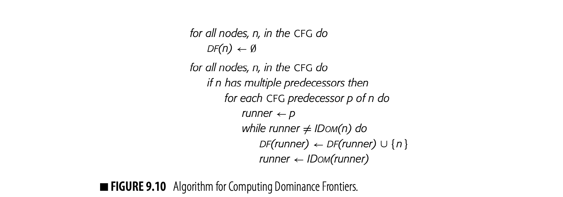
To make $\varphi$-insertion efficient, the compiler should precompute, for each CFG node $n$, a set $\text{DF}(n)$ that contains $n$'s dominance frontier. The algorithm, shown in Fig. 9.10, uses both the dominator tree and the CFG to build the $\text{DF}(n)$ sets.

Notice that the DF sets can only contain nodes that are join points in the CFG--that is, nodes that have multiple predecessors. Thus, the algorithm starts with the join points. At a CFG join point $n$, it iterates over $n$'s CFG predecessors $p$ and inserts $n$ into $\text{DF}(p)$ as needed.

If $p=\mathrm{IDom}(n)$, then p also dominates all of n 's other predecessors. In the example, $B_0=\mathrm{IDom}\left(B_1\right)$.

• If $p=\text{IDom}(n)$, then $n$ does not belong to $\text{DF}(p)$. Neither does it belong to $\text{DF}(m)$ for any predecessor $m$ of $p$.
• If $p\ne \text{IDom}(n)$, then $n$ belongs in $\text{DF}(p)$. It also belongs in $\text{DF}(q)$ for any $q$ such that $q\in \text{Dom}(p)$ and $q\notin (\text{Dom}(n)-n)$. The algorithm finds these latter nodes $q$ by running up the dominator tree.

The algorithm follows from these observations. It initializes $\text{DF}(n)$ to $\varnothing$, for all CFG nodes $n$. Next, it finds each CFG join point $n$ and iterates over $n$'s

CFG predecessors, $p$. If $p$ dominates $n$, the algorithm is done with $p$. If not, it adds $n$ to DF($p$) and walks up the dominator tree, adding $n$ to the DF set of each dominator-tree ancestor until it finds $n$'s immediate dominator. The algorithm needs a small amount of bookkeeping to avoid adding $n$ to a DF set multiple times. Consider again the example CFG and its dominator tree. The analyzer examines the nodes in some order, looking for nodes with multiple predecessors. Assuming that it takes the nodes in name order, it finds the join points as $B_1$, then $B_3$, then $B_7$.

• For CFG-predecessor $B_0$, the algorithm finds that $B_0$ is IDom($B_1$), so it never enters the while loop. For CFG-predecessor $B_3$, it adds $B_1$ to DF($B_3$) and sets $runner$ to IDom($B_3$) = $B_1$. It adds $B_1$ to DF($B_1$) and sets $runner$ to IDom($B_1$) = $B_0$, where it halts.
• For CFG-predecessor $B_2$, it adds $B_3$ to DF($B_2$) and sets $runner$ to IDom($B_2$) = $B_1$. Since $B_1$ = IDom($B_3$), it halts. For CFG-predecessor $B_7$, it adds $B_3$ to DF($B_7$) and sets $runner$ to IDom($B_7$) = $B_5$. It adds $B_3$ to DF($B_5$) and sets $runner$ to IDom($B_5$) = $B_1$, where it halts.
• For CFG-predecessor $B_6$, it adds $B_7$ to DF($B_6$) and advances $runner$ to IDom($B_6$) = $B_5$, where it halts. For CFG-predecessor $B_8$, it adds $B_7$ to DF($B_8$) and advances $runner$ to IDom($B_8$) = $B_5$, where it halts.

These results produce the DF sets shown in the table in Fig. 9.9.

9.3.3 Placing $\varphi$-Functions

The naive algorithm placed a $\varphi$-function for every variable at the start of every join node. With dominance frontiers, the compiler can determine more precisely where $\varphi$-functions might be needed. The basic idea is simple.

• From a control-flow perspective, an assignment to $x$ in CFG node $n$ induces a $\varphi$-function in every CFG node m\in\mbox{DF}(n). Each inserted $\varphi$-function creates a new assignment; that assignment may, in turn, induce additional $\varphi$-functions.
• From a data-flow perspective, a $\varphi$-function is only necessary if its result is live at the point of insertion. The compiler could compute live information and check each $\varphi$-function on insertion; that approach leads to pruned SSA form.

The word $global$ is used here to mean of interest across the entire procedure.

In practice, the compiler can avoid most dead $\varphi$-functions with an inexpensive approximation to liveness. A name $x$ cannot need a $\varphi$-function unless it is live in multiple blocks. The compiler can compute the set of global names--those that are live in multiple blocks. The SSA-construction can ignore any nonglobal name, which reduces the name space and the number of $\varphi$-functions. The resulting SSA form is called $\text{semipruned SSA form}$.

The compiler can find the global names cheaply. In each block, it looks for names with upward-exposed uses--the UEVar set from the live-variables calculation. Any name that appears in a LiveOut set must be in the UEVar set of some block. Taking the union of all the UEVar sets gives the compiler the set of names that are live on entry to one or more blocks and, hence, live in multiple blocks.

The algorithm to find global names, shown in Fig. 11(a), is derived from the obvious algorithm for computing UEVar. It constructs both a set of global names, Globals, and, for each name, the set of blocks that contain a definition of that name. The algorithm uses these block lists to form initial worklists during $\varphi$-function insertion.

The algorithm for inserting $\varphi$-functions, in panel (b), iterates over the global names. For each name $x$, it initializes WorkList with Blocks($\varphi$). For each block $b$ in WorkList, it inserts a $\varphi$-function at the head of each block $d$ in $b$'s dominance frontier. The parallel execution semantics of the $\varphi$-functions lets the algorithm insert them at the head of $d$ in any order. When it adds a $\varphi$-function for $x$ to $d$, the algorithm adds $d$ to WorkList to reflect the new assignment to $x$ in $d$.

Example

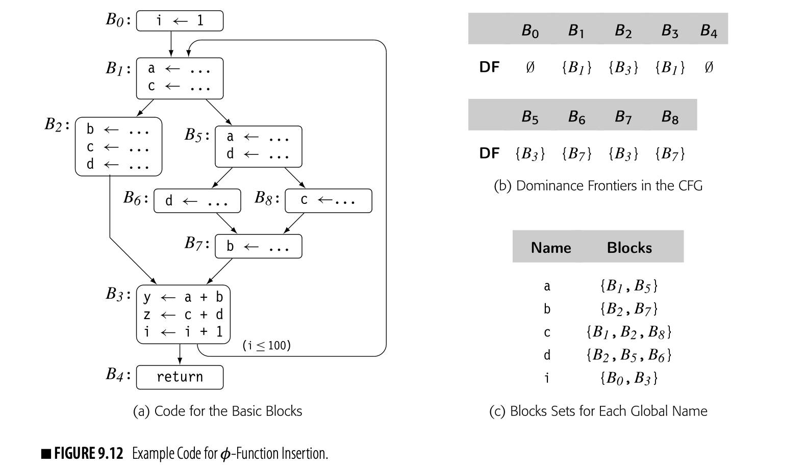
Fig. 9.12 recaps our running example. Panel (a) shows the code and panel (b) shows the dominance frontiers for the CFG.

The compiler could avoid computing Blocks sets for nonglobal names, at the cost of another pass over the code.

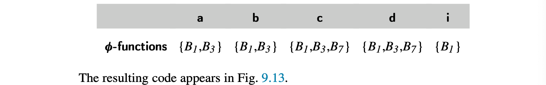
The first step in the $\varphi$-function insertion algorithm finds global names and computes the $Blocks$ set for each name. The global names are $\{\text{a},\text{b},\text{c},\text{d},\text{i}\}$. The $Blocks$ sets for the global names are shown in panel (c). While the algorithm computes a $Blocks$ set for each of y and z, the table omits them because they are not global names.

The $\varphi$-function insertion algorithm, shown in Fig. 9.11(b), works on a name-by-name basis. Consider its actions for the variable a in the example. First, it initializes the worklist to $Blocks(\text{a})=\{B_I,B_S\}$, to denote the fact that a is defined in $B_I$ and $B_S$.

The definition of a in $B_I$ causes insertion of a $\varphi$-function for a at the start of each block in $\mathrm{DF}(B_I)=\{B_I\}$. The $\varphi$-function in $B_I$ is a new assignment, so the algorithm adds $B_I$ to $Worklist$. Next, the algorithm removes $B_S$ from the worklist and inserts a $\varphi$-function in each block of $\mathrm{DF}(B_S)=\{B_S\}$. The new $\varphi$-function in $B_S$ causes the algorithm to add $B_S$ to the worklist. When $B_I$ comes off the worklist, the algorithm discovers that the $\varphi$-function induced by $B_I$ in $B_I$ already exists. It neither adds a duplicate $\varphi$-function nor adds blocks to $Worklist$. When $B_S$ comes off the worklist, the algorithm also finds the $\varphi$-function for a in $B_I$. At that point, $Worklist$ is empty and the processing for a halts.

The algorithm follows the same logic for each name in Globols, to produce the following insertions:

Limiting the algorithm to global names keeps it from inserting dead $\varphi$-functions for $y$ and $z$ in block $B_I$. ($B_I\in \mathrm{DF}(B_3)$ and $B_3$ defines both $y$ and $z$.) However, the distinction between local names and global names is not sufficient to avoid all dead $\varphi$-functions. For example, the $\varphi$-function for b in $B_I$ is not live because b is redefined before its value is used. To avoid inserting these $\varphi$-functions, the compiler can construct LiveOut sets and add a test based on liveness to the inner loop of the $\varphi$-function insertion algorithm. That modification causes the algorithm to produce $\text{pruned SSA form}$.

Efficiency Improvements

To improve efficiency, the compiler should avoid two kinds of duplication. First, the algorithm should avoid placing any block on the worklist more than once per global name. It can keep a checklist of blocks that have already been processed for the current name and reset the checklist when it starts to process a new name.

Both of these checklists can be imple- mented as sparse sets (see Appendix B.2.3).

Second, a given block can be in the dominance frontier of multiple nodes that appear on the WorkList. The algorithm must check, at each insertion, for a preexisting $\varphi$-function for the current name. Rather than searching through the $\varphi$-functions in the block, the compiler should maintain a checklist of blocks that already contain $\varphi$-functions for the current variable. Again, this checklist must be reset when the algorithm starts to process a new name.

9.3.4 Renaming

Earlier, we stated that the algorithm for renaming variables was conceptually straightforward. The details, however, require explanation.

In the final SSA form, each global name becomes a base name, and individual definitions of that base name are distinguished by the addition of a numerical subscript. For a name that corresponds to a source-language variable, say a, the algorithm uses a as the base name. Thus, the first definition of a that the renaming algorithm encounters will be named a0 and the second will be a1. For a compiler-generated temporary, the algorithm can use its pre-SSA name as its base name.

The algorithm, shown in Fig. 14, renames both definitions and uses in a preorder walk over the procedure's dominator tree. In each block, it first renames the values defined by $\varphi$-functions at the head of the block. Next, it visits each operation in the block, in order. It rewrites the operands with current SSA names and then creates a new SSA name for the result of the operation. This latter act makes the new name current. After all the operations in the block have been rewritten, the algorithm rewrites the appropriate $\varphi$-function parameters in each CFG successor of the block, using the current SSA names. Finally, it recurs on any children of the block in the dominator tree. When it returns from those recursive calls, it restores the set of current SSA names to the state that existed before the current block was visited.

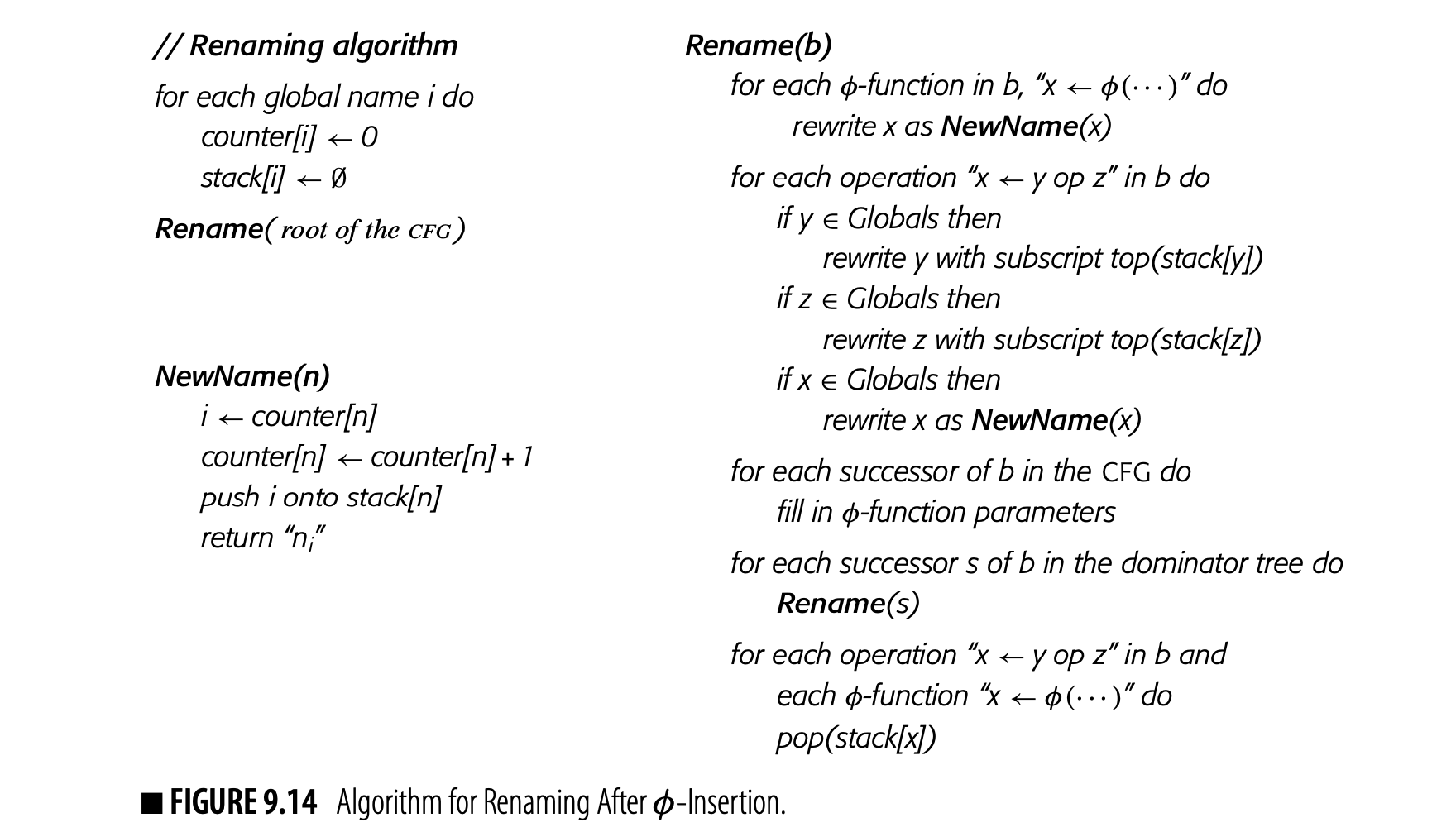
To manage the names, the algorithm uses a counter and a stack for each global name. A name's stack holds the subscript from its current SSA name. At each definition, the algorithm generates a new subscript for the defined base name by pushing the value of its current counter onto the stack and incrementing the counter. Thus, the value on top of the stack for $n$ is always the subscript of $n$'s current SSA name.

As the final step, after recurring on the block's children in the dominator tree, the algorithm pops all the names generated in that block off their respective stacks. This action reveals the names that held at the end of that block's immediate dominator. Those names may be needed to process the block's remaining dominator-tree siblings.

The stack and the counter serve distinct and separate purposes. As the algorithm moves up and down the dominator tree, the stack is managed to simulate the lifetime of the most recent definition in the current block. The counter, on the other hand, grows monotonically to ensure that each successive definition receives a unique SSA name.

Fig. 9.14 summarizes the algorithm. It initializes the stacks and counters, then calls Rename on the dominator tree's root--the CFG's entry node. Rename processes the block, updates $\varphi$-function arguments in its CFG successor blocks, and recurs on its dominator-tree successors. To finish the block, Rename pops off the stacks any names that it added as it processed the block. The function NewName manipulates the counters and stacks to create new SSA names as needed.

One final detail remains. When Rename rewrites the $\varphi$-function parameters in each of $b$'s CFG successors, it needs a mapping from $b$ to an ordinal parameter slot in those $\varphi$-functions for $b$. That is, it must know which parameter slot in the $\varphi$-functions corresponds to $b$.

When we draw SSA form, we assume a left-to-right order that matches the left-to-right order in which the edges are drawn. Internally, the compiler can number the edges and parameter slots in any consistent fashion that produces the desired result. This requires cooperation between the code that builds SSA and the code that builds the CFG. (For example, if the CFG implementation uses a list of edges leaving each block, the order of that list can determine the mapping.)

Example

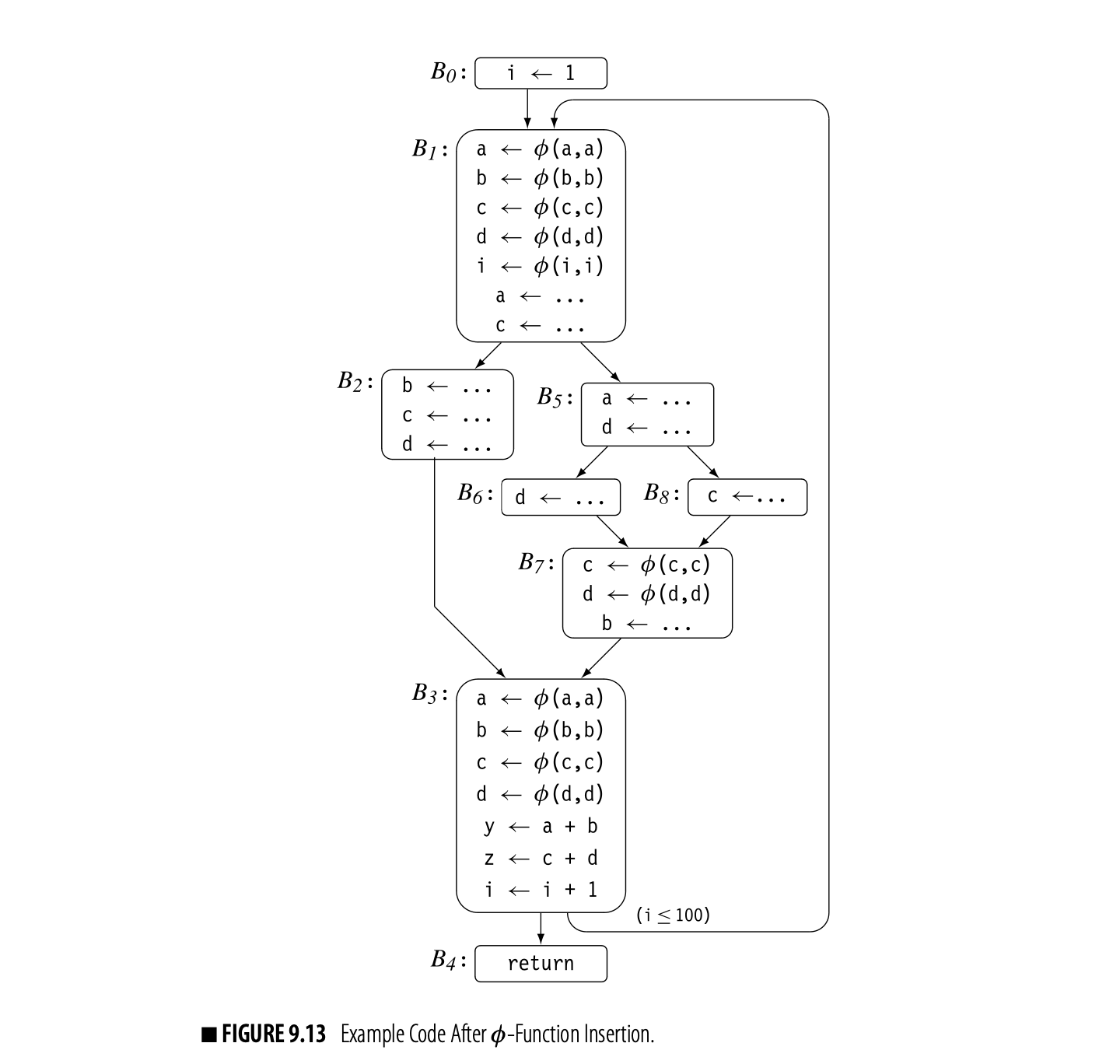
To finish the continuing example, let's apply the renaming algorithm to the code in Fig. 9.13. Assume that $a_0$, $b_0$, $c_0$, and $d_0$ are defined on entry to $B_0$. Fig. 9.15 shows the states of the counters and stacks for global names at various points during the process.

The algorithm makes a preorder walk over the dominator tree, which, in this example, corresponds to visiting the nodes in ascending order by name. Fig. 9.15(a) shows the initial state of the stacks and counters. As the algorithm proceeds, it takes the following actions:

Block $B_0$ This block contains only one operation. Rename rewrites $i$ with $i_0$, increments $i$'s counter, and pushes $i_0$ onto the stack for $i$. Next, it visits $B_0$'s CFG-successor, $B_I$, and rewrites the $\varphi$-function parameters that correspond to $B_0$ with their current names: $a_0$, $b_0$, $c_0$, $d_0$, and $i_0$. It then recurs on $B_0$'s child in the dominator tree, $B_I$. After that, it pops the stack for $1$ and returns.

Block $B_1$ Rename enters $B_I$ with the state shown in panel (b). It rewrites the $\varphi$-function targets with new names, $a_1$, $b_1$, $c_1$, $d_1$, and $i_1$. Next, it creates new names for the definitions of $a$ and $c$ and rewrites them. Neither of $B_I$'s CFG successors have $\varphi$-functions, so it recurs on $B_I$'s dominator-tree children, $B_2$, $B_3$, and $B_5$. Finally, it pops the stacks and returns.

Block $B_2$ Rename enters $B_2$ with the state shown in panel (c). This block has no $\varphi$-functions to rewrite. Rename rewrites the definitions of $b$, $c$, and $d$, creating a new SSA name for each. It then rewrites $\varphi$-function parameters in $B_2$'s CFG successor, $B_3$. Panel (d) shows the stacks and counters just before they are popped. Finally, it pops the stacks and returns.

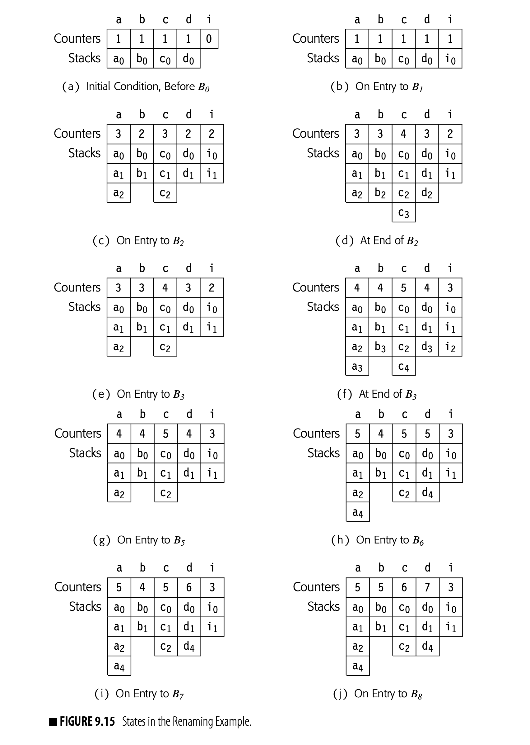
Block B3 Rename enters $B_3$ with the state shown in panel (e). Notice that the stacks have been popped to their state when Rename entered $B_2$, but the counters reflect the names created inside $B_2$. In $B_3$, Rename rewrites the $\varphi$-function targets, creating new SSA names for each. Next, it rewrites each assignment in the block, using current SSA names for the uses of global names and then creating new SSA names for definitions of global names. $B_3$ has two CFG successors, $B_1$ and $B_4$. In $B_1$, it rewrites the $\varphi$-function parameters that correspond to the edge from $B_3$, using the stacks and counters shown in panel (f). $B_4$ has no $\varphi$-functions. Next, Rename recurs on $B_3$'s dominator-tree child, $B_4$. When that call returns, Rename pops the stacks and returns.

Block B4 This block just contains a return statement. It has no $\varphi$-functions, definitions, uses, or successors in either the CFG or the dominator tree. Thus, Rename performs no actions and leaves the stacks and counters unchanged.

Block B5 After $B_4$, Rename pops through $B_3$ back to $B_1$. With the stacks as shown in panel (g), it recurs down into $B_1$'s final dominator-tree child, $B_5$. $B_5$ has no $\varphi$-functions. Rename rewrites the two assignment statements, creating new SSA names as needed. Neither of $B_5$'s CFG successors has $\varphi$-functions. Rename next recurs on $B_5$'s dominator-tree children, $B_6$, $B_7$, and $B_8$. Finally, it pops the stacks and returns.

Block B6 Rename enters $B_6$ with the state in panel (h). $B_6$ has no $\varphi$-functions. Rename rewrites the assignment to d, generating the new SSA name d5. Next, it visits the $\varphi$-functions in $B_6$'s CFG successor $B_7$. It rewrites the $\varphi$-function arguments along the edge from $B_6$ with their current names, $c_2$ and d5. Since $B_6$ has no dominator-tree children, it pops the stack for d and returns.

Block B7 Rename enters $B_7$ with the state shown in panel (i). It first renames the $\varphi$-function targets with new SSA names, $c_5$ and d6. Next, it rewrites the assignment to b with new SSA name b4. It then rewrites the $\varphi$-function arguments in $B_7$'s CFG successor, $B_3$, with their current names. Since $B_7$ has no dominator-tree children, it pops the stacks and returns.

Block B8: Rename enters $B_8$ with the state shown in panel (j). $B_8$ has no $\varphi$-functions. Rename rewrites the assignment to c with new SSA name c6. It rewrites the appropriate $\varphi$-function arguments in $B_7$ with their current names, $c_6$ and d4. Since $B_8$ has no dominator-tree children, it pops the stacks and returns.

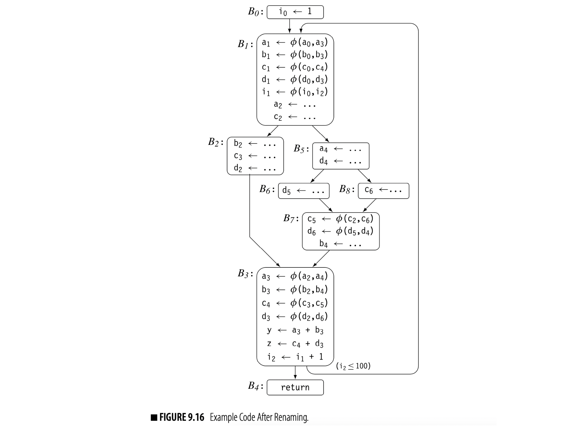
Fig 9.16 shows the code after Rename halts.

A Final Improvement

We can reduce the time and space spent in stack manipulation with a clever implementation of NewName. The primary use of the stacks is to reset the name space on exit from a block. If a block redefines the same base name multiple times, the stack only needs to keep the most recent name. For example, in block $B_I$, both a and c are defined twice. NewName could reuse the slots for a${}_1$ and c${}_1$ when it creates a${}_2$ and c${}_2$.

With this change, Rename performs one push and one pop per base name defined in the block. NewName can keep a list of the stack entries that it creates; on exit from the block, Rename can then walk the list to pop theappropriate stacks. The stacks require less space; their size is bounded by the depth of the dominator tree. Stack manipulation is simplified; the algorithm performs fewer push and pop operations and the push operation need not test for a stack overflow.

9.3.5 Translation out of SSA Form

Actual processors do not implement φ- functions, so the compiler must rewrite the code without the φ-functions.

A compiler that uses SSA form must translate that form of the code back into a more conventional model--one without $\varphi$-functions--before the code can execute on conventional computer hardware. The compiler must replace the $\varphi$-functions with copy operations and place them in the code so that they reproduce the semantics of those $\varphi$-functions: both the control-based selection of values and the parallel execution at the start of the block.

This section addresses out-of-SA translation. It begins with an overly simple, or naive, translation, which informs and motivates the actual translation schemes. Next, it presents two example problems that demonstrate the problems that can arise in translating from SSA form back to conventional code. Finally, it presents a unified framework that addresses the known complexities of the translation.

The Naive Translation

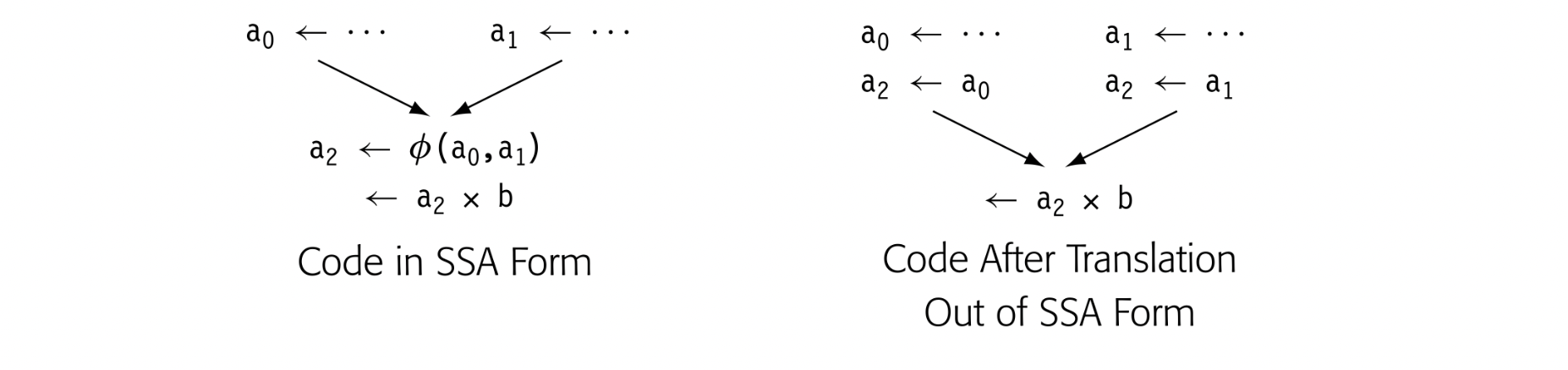
A $\varphi$-function is just a copy operation that selects its input based on prior control-flow. To replicate the effect of a $\varphi$-function at the top of block $b$, the compiler can insert, at the end of each CFG-predecessor of $b$, a copy operation that moves the appropriate $\varphi$-function argument into the name defined by the $\varphi$-function (shown in the margin). Once the compiler has inserted the copies, it can delete the $\varphi$-function.

This process, while conceptually simple, has some complications. Consider, for example, the continuing example from Fig. 16. Three blocks in the CFG contain $\varphi$-functions: $B_1$, $B_3$, and $B_7$. Fig. 17 shows the code after copies have been inserted.

For $B_3$ and $B_7$, insertion into the predecessor blocks works. The predecessors of both $B_3$ and $B_7$ have one successor each, so the copy operations inserted at the end of those predecessor blocks have no effect on any path other than the one to the $\varphi$-function.

The situation is more complex for $B_1$. Copy insertion at the end of $B_1$'s predecessor, $B_0$, produces the desired result; the copies only occur on the path $(B_0,B_1)$. With $B_1$'s other predecessor, $B_3$, simple insertion will not work. A copy inserted at the end of $B_3$ will execute on both $(B_3,B_1)$ and $(B_3,B_4)$. Along $(B_3,B_4)$, the copy operation may change a value that is live in $B_4$.

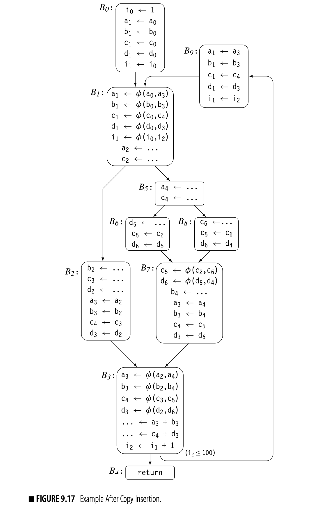
Critical edge A flow graph $edge(i,j)$ is a critical edge if $i$ has multiple successors and $j$ has multiple predecessors. Optimizations that move or insert code often need to split critical edges.

The edge $(B_3,B_1)$ highlights a more general problem with code placement on a critical edge. $B_3$ has multiple successors, so the compiler cannot insert the copy at the end of $B_3$. $B_1$ has multiple predecessors, so the compiler cannot insert the copy at the start of $B_I$. Since neither solution works, the compiler must split the edge and create a new block to hold the inserted copy operations. With the split edge and the creation of $B_9$, the translated code faithfully reproduces the effects of the SSA form of the code.

Problems with the Naive Translation

If the compiler applies the naive translation to code that was produced directly by the translation into SSA form, the results will be correct, as long as critical edges can be split. If, however, the compiler transforms the code while it is in SSA form--particularly, transformations that move definitions or uses of SSA names--or if the compiler cannot split critical edges, then the naive translation can produce incorrect code. Two examples demonstrate how the naive translation can fail.

The Lost-Copy Problem

In Fig. 9.17, the compiler had to split the edge $(B_3,B_1)$ to create a location for the copy operations associated with that edge. In some situations, the compiler cannot or should not split a critical edge. For example, an SSA-based register allocator should not add any blocks or edges during copy insertion (see Section 13.5.3). The combination of an unsplit critical edge and an optimization that extends some SSA-name's live range can create a situation where naive copy insertion fails.

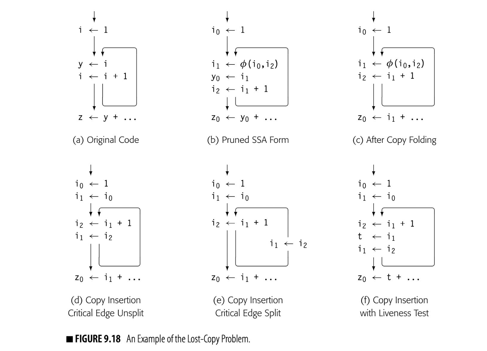
Fig. 9.18(a) shows an example to demonstrate the problem. The loop increments $i$. The computation of $z$ after the loop uses the second-to-last value of $i$. Panel (b) shows the pruned SSA for the code.

Panel (c) shows the code after copy folding. The use of $y_0$ in the computation of $z_0$ has been replaced with a use of $i_1$. The last use of $i_1$ in panel (b) was in the assignment to $y_0$; folding the copy extends the live range of $i_1$ beyond the end of the loop in panel (c).

Copy folding an optimization that removes unneeded copy operations by renaming the source and destination to the same name, when such renaming does not change the flow of values $\text{Copy folding}$ is also called $\text{copy coalescing}$ (see Section 13.4.3).

Copy insertion on the code in panel (c) adds $i_1\leftarrow i_0$ to the end of the preloop block, and $i_1\leftarrow i_2$ at the end of the loop. Unfortunately, that latter assignment kills the value in $i_1$; the computation of $z_0$ now receives the final value of $i$ rather than its penultimate value. Copy insertion produces incorrect code because it extends $i_1$'s live range.

Splitting the critical edge cures the problem, as shown in panel (e); the copy does not execute on the loop's final iteration. When the compiler cannot split that edge, it must add a new name to preserve the value of $i_1$, as shown in panel (f). A simple, ad-hoc addition to the copy insertion process can avoid the lost-copy problem. As the compiler inserts copies, it should check whether or not the target of the new copy is live at the insertion point. If the target is live, the compiler must introduce a new name, copy the live value into it, and propagate that name to the uses after the insertion point.

The Swap Problem

The concurrent semantics of $\varphi$-functions create another problem for out-of-SSA translation, which we call the swap problem. The motivating example appears in Fig. 9.19(a): a simple loop that repeatedly swaps the values of $x$ and $y$. If the compiler builds pruned SSA-form, as in panel (b), and performs copy folding, as in panel (c), it creates a valid program in SSA form that relies directly on the concurrent semantics of the $\varphi$-functions in a single block.

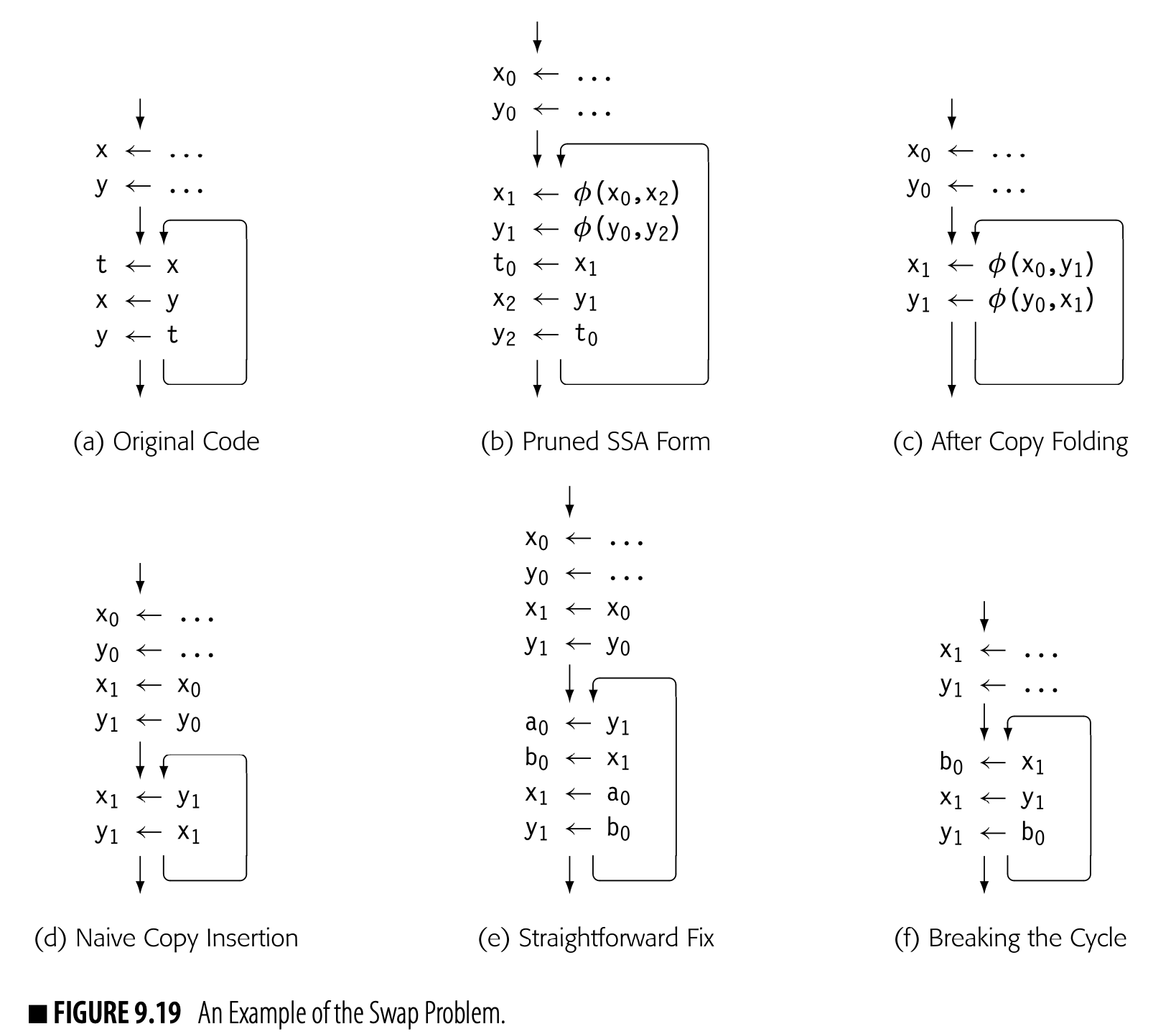
Because the two $\varphi$-functions read their values concurrently and then write their results concurrently, the code in panel (c) has the same meaning as theoriginal code from panel (a). Naive copy-insertion, however, replaces each $\varphi$-function with a sequential copy operation, as shown in panel (d). The two sequential copies have a different result than did the two $\varphi$-functions; the substitution fundamentally changes the meaning of the code.

To maintain the original code's meaning, the compiler must ensure that the inserted copies faithfully reproduce the flow of values specified by the $\varphi$-functions. Thus, it must pay attention to any values that are defined by one $\varphi$-function and used by another $\varphi$-function in the same block.

In some cases, the compiler must introduce one or more new names. The straightforward solution to this problem is to adopt a two-stage copy protocol, as shown in panel (e). The first stage copies each of the $\varphi$-function arguments into its own temporary name, simulating the control-based selection and the parallel read of the $\varphi$-function. The second stage then copies those values to the $\varphi$-function targets.

Unfortunately, this solution doubles the number of copy operations required to translate out of SSA form. The compiler can reduce the number of temporary names and extra copy operations by building a small dependence graph for the set of parallel copies implied by the $\varphi$-functions and using the graph to guide insertion of the sequential copies. If the dependence graph is acyclic, then the compiler can use it to schedule the copy operations in a way that requires no additional names or operations (see Chapter 12).

If the dependence graph contains cycles, then the compiler must break each cycle with a copy into a name not involved in the cycle. This may require a new name. The dependence graph for the example, shown in the margin, consists of a two node cycle. It requires one new name to break the cycle, which produces the code shown in panel (f).

A Unified Approach to Out-of-SSA Translation

The swap problem and the copy problem arise from two distinct phenomena: transformations that change the range over which an SSA-name is live, and failure to preserve the parallel semantics of $\varphi$-function execution during translation out of SSA-form. Common code transformations, such as copy folding, code motion, and cross-block instruction scheduling, can create the circumstances that trigger these problems. While the solutions proposed in the previous section will generate correct code, neither solution provides a clean framework for understanding the underlying issues.

The unified approach uses a three-phase plan to address the two issues caused by code transformations on the SSA form: changes in the live ranges of SSA names and implicit use of the parallel semantics of $\varphi$-function execution. Phase one introduces a new set of names to isolate $\varphi$-functions from the rest of the code; it then inserts parallel copy operations to connect those names with the surrounding context. Phase two replaces $\varphi$-functions with parallel copy operations in predecessor blocks. Phase three rewrites each block of parallel copies with an equivalent series of sequential copies. This process avoids both the swap problem and the lost copy problem. At the same time, it eliminates the need to split critical edges.

Phase One

We will denote a parallel copy group by adding a common subscript to the assignment operator, ${\leftarrow }_i$.

To isolate the name space for a $\varphi$-function, such as ${\mathtt{a}}_0\leftarrow \varphi ({\mathtt{a}}_1,{\mathtt{a}}_2,\dots ,{\mathtt{a}}_n)$, phase one rewrites it as ${\mathtt{a}}_0^{\prime }\leftarrow \varphi \left({\mathtt{a}}_1^{\prime },{\mathtt{a}}_2^{\prime },\dots ,{\mathtt{a}}_n^{\prime }\right)$. To connect the new primed names with the surrounding code, the compiler adds a copy operation ${\mathtt{a}}_i^{\prime }\leftarrow {\mathtt{a}}_i$ to the end of the predecessor block associated with ${\mathtt{a}}_i$, for each parameter ${\mathtt{a}}_i$. To retain the parallel execution semantics of the $\varphi$-functions, the compiler will use parallel copy groups for the copies that it inserts.

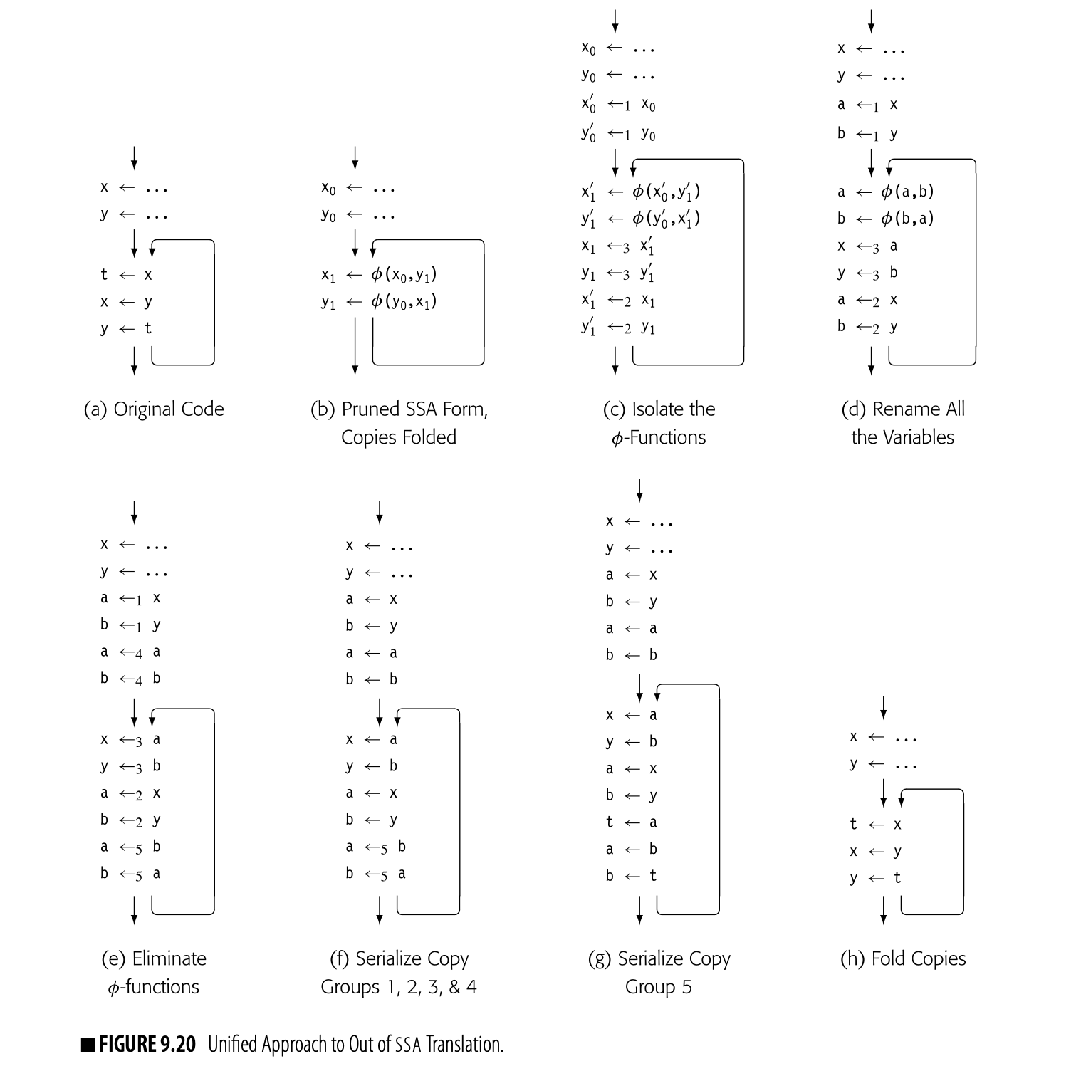
After the group of $\varphi$-functions at the head of a block, the compiler should insert another parallel copy group. For each $\varphi$-function in the block, ${\mathsf{a}}_{\mathsf{i}}\leftarrow \varphi (\dots )$, the copy group should include a copy of the form ${\mathsf{a}}_{\mathsf{i}}\leftarrow {\mathsf{a}}_{\mathsf{i}}^{\prime }$. The net effect of these three actions is to isolate the names used in the $\varphi$-functions from the surrounding code and to make the impact of parallel execution explicit, outside of the $\varphi$-functions. Fig. 9.20 shows the effects of this transformation on the example from the swap problem. Panel (a) shows the original code; panel (b) shows it in pruned ssa form, with copies folded. Panel (c) shows the code after the compiler has isolated the $\varphi$-functions. The $\varphi$-function parameters have been renamed and parallel copy groups inserted.

• Parallel copy group 1, at the end of the first block, gives $x_0^{\prime }$ and $y_0^{\prime }$ their initial values.
• Parallel copy group 2, at the end of the loop body, gives $x_1^{\prime }$ and $y_1^{\prime }$ their values from computation inside the loop. (The loop body is its own predecessor.)
• Parallel copy group 3, after the $\varphi$-functions, copies the values defined by the $\varphi$-functions into the names that they had before the renaming transformation. At this point, the compiler can rename all of the primed variables and drop all of the subscripts from SSA names, as shown in panel (d). The renamed code retains the meaning of the original code.

Phase Two

This phase replaces $\varphi$-functions by inserting copies into predecessor blocks and deleting the $\varphi$-functions. To retain the $\varphi$-function semantics, the compiler uses parallel copies in each block.

At the end of phase one as shown in panel (d), the actual value swap occurs during evaluation of the $\varphi$-function arguments. After $\varphi$-function replacement, shown in panel (e), that value swap occurs in parallel copy group 5, at the end of the loop body.

At the end of phase two, the compiler has eliminated all of the $\varphi$-functions. The code still contains groups of parallel copy operations that implement the semantics of the $\varphi$-functions. To complete the process, the compiler must rewrite each parallel copy group into a set of serial copies. The code will likely contain multiple (perhaps many) unneeded copy operations. Coalescing can eliminate some or all of them (see Section 13.4.3).

Phase Three

The final phase examines each parallel copy group and rewrites it with an equivalent group of sequential copy operations. It builds a data-dependence graph for the copy group (see Section 4.3.2). If the graph is acyclic, as in the acyclic graph shown in the margin, the compiler can simply insert copies in the order implied by the graph--leaves to roots. For the first example, the graph requires that $a\leftarrow b$ and $d\leftarrow b$ precede $b\leftarrow c$. If the dependence graph contains a cycle, as shown in the example in the margin, the compiler must insert copies in a way that breaks the cycle. In the example, it must copy one of the values, say a, into a new temporary name, say t. Then, it can perform a $\leftarrow$ b and b $\leftarrow$ c. It can finish the copy group with c $\leftarrow$ t. This breaks the cycle and correctly implements the semantics of teh parallel copy group. In some cases, the compiler can avoid the new name by careful ordering. For example, if the second example also included a copy d ${\leftarrow }_2$ a, the compiler could schedule d $\leftarrow$ a first and break the cycle by rewriting c $\leftarrow$ a as c $\leftarrow$ d.

In the example, groups 1, 2, 3, and 4 can be serialized without additional names, as shown in panel (f). Copy group 5 contains a cycle, so it requires one new name, t. Panel (g) shows the rewrite of copy group 5. Panel (h) shows the final code after copy folding.

9.3.6 Using SSA Form

A compiler writer uses SSA form because it improves the quality of analysis, the quality of optimization, or both. To see how analysis on SSA differs from the classical data-flow analysis techniques presented in Section 9.2, consider the problem of global constant propagation on SSA, using an algorithm called sparse simple constant propagation (SSCP).

Semilattice a set $L$ and a $meet$ operator $\wedge$ such that, $\forall$ a, b, and $c\in L$,

1. $a\wedge a=a$,
2. $a\wedge b=b\wedge a$, and
3. $a\wedge (b\wedge c)=(a\wedge b)\wedge c$ Compilers use semilattices to model the data domains of analysis problems.

In SSCP, the compiler annotates each SSA name with a value. The set of possible values forms a semilattice. A semilattice consists of a set $L$ of values and a meet operator, $\wedge$. The meet operator must be idempotent, commutative, and associative; it imposes an order on the elements of $L$:

Every semilattice has a bottom element, $\perp$, with the properties that Some semilattices also have a top element, $\top$, with the properties that In constant propagation, the structure of the semilattice used to model program values plays a critical role in the algorithm's runtime complexity. The semilattice for a single SSA name appears in the margin. It consists of $\top$, $\perp$, and an infinite set of distinct constant values. For any value $x$: $x\wedge \top =x$, and $x\wedge \perp =\perp$. For two constants, $c_i$ and $c_j$: $c_i\wedge c_j=\perp$ if $c_i\ne c_j$. If $c_i=c_j$, then $c_i\wedge c_j=c_i$.

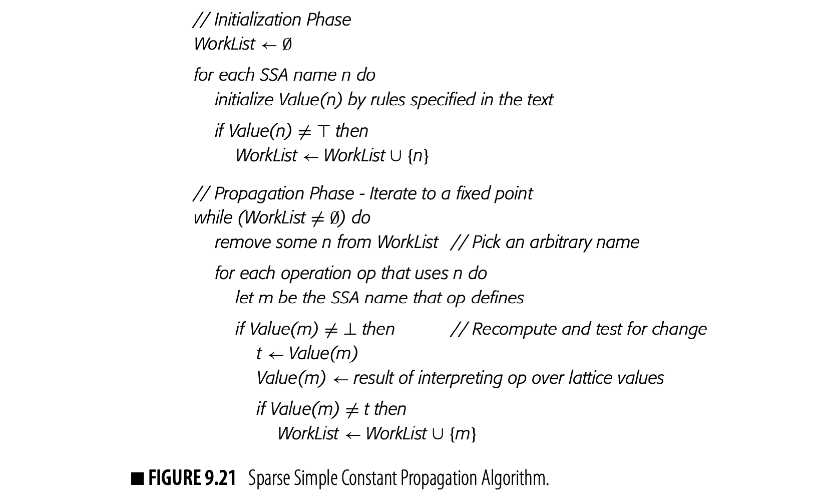The algorithm for SSCP, shown in Fig. 9.21, consists of an initialization phase and a propagation phase. The initialization phase iterates over the SSA names. For each SSA name $n$, it examines the operation that defines $n$ and sets $\text{Value(n)}$ according to a simple set of rules.

1. If n is defined by a \phi-function, \operatorname{SSCP} sets \operatorname{Value}(n) to T.
2. if n 's value is not known, \operatorname{SSCP} sets \operatorname{Value}(n) to T.
3. If n 's value is a known constant c_{i}, \operatorname{SSCP} sets Value (n) to c_{i}.
4. If n 's value cannot be known-for example, it is defined by reading a value from external media—SSCP sets \operatorname{Value}(n) to \perp.

If Value (n) is not T, the algorithm adds n to the worklist.

These initializations highlight the use of T and $\perp$ in the constant propagation semilattice. T indicates that the compiler does not yet know anything about the value, but that it might discover information about its value in the future. By contrast, $\perp$ indicates that the compiler has proven that the value is not a constant. For any SSA name m, $\text{Value(m)}$ can change at most twicethe height of the semilattice. If $\text{Value(m)}$ starts as $\mathrm{T}$, it can progress to some constant $c_i$ or to $\perp$. If $\text{Value (m)}$ is some constant $c_i$, it can progress to $\perp$. Once $\text{Value(m)}$ is $\perp$, it cannot change.

The propagation phase is straightforward. It removes an SSA name n from the worklist. The algorithm examines each operation op that uses n, where op defines some SSA name m. If $\text{Value(m)}$ has already reached $\perp$, then no further evaluation is needed. Otherwise, it models the evaluation of op by interpreting the operation over the lattice values of its operands. If the result is lower in the lattice than $\text{Value(m)}$, it lowers $\text{Value(m)}$ accordingly and adds m to the worklist. The algorithm halts when the worklist is empty.

Interpreting an operation over lattice values requires some care. For a $\varphi$-function, the result is simply the meet of the lattice values of all the $\varphi$-function's arguments; the rules for meet are shown in the margin, in order of precedence. For other kinds of operations, the compiler needs a set of rules. Consider, for example, $a\times b$. If $a=4$ and $b=17$, then $a\times b=68$. However, if $a=\perp$, then $a\times b=\perp$, unless $b=0$. ($a\times 0=0$, for any $a$.)

In general, the evaluation rules for operators should preserve $\top$, unless the other operand forces a value, as with multiplication by zero. If $a=\top$, then evaluating $a+b$ to $\top$ will defer determination of the sum until $a$'s value is resolved to either a constant or $\perp$.

Complexity

The propagation phase of SSCP is a classic fixed-point scheme. The arguments for termination and complexity follow from the length of descending chains through the semilattice, shown again in the margin. The lattice value for an SSA name can change at most twice: from $\top$ to ${\mathsf{c}}_1$ and from ${\mathsf{c}}_1$ to $\perp$. SSCP only adds an SSA name to the worklist when its value changes, so each name appears on the worklist at most twice. SSCP evaluates an operation when one of its operands is removed from the worklist, which bounds the number of evaluations at twice the number of uses in the code.

Optimism: The Role of Top

As discussed earlier, SSCP uses the lattice value $\top$ to represent a lack of knowledge. This practice differs from the data-flow problems in Section 9.2, which use the value $\perp$ but not the value $\top$. The use of $\top$ as an initial value plays a critical role in constant propagation; it allows values to propagate into cycles in the graph.

Because it initializes unknown values to $\top$, rather than $\perp$, it can propagate some values into cycles in the graph--loops in the CFG. Algorithms that begin with the value $\top$, rather than $\perp$, are often called optimistic algorithms. The intuition behind "optimism" is that initialization to $\top$ allows the algorithm to propagate information into a cyclic region, optimistically assuming that the value along the back edge will confirm this initial propagation. An initialization to $\perp$, called pessimistic, disallows that possibility.

Consider the SSA fragment in Fig. 9.22. If the algorithm initializes ${\mathsf{x}}_1$ and ${\mathsf{x}}_2$ to $\perp$ (pessimism), it will not propagate the value $17$ into the loop. When it evaluates the $\varphi$-function, it sets $x_1$ to $17\wedge \perp =\perp$. Once $x_1=\perp$, propagation sets $x_2=\perp$, independent of $i_{12}$'s value.

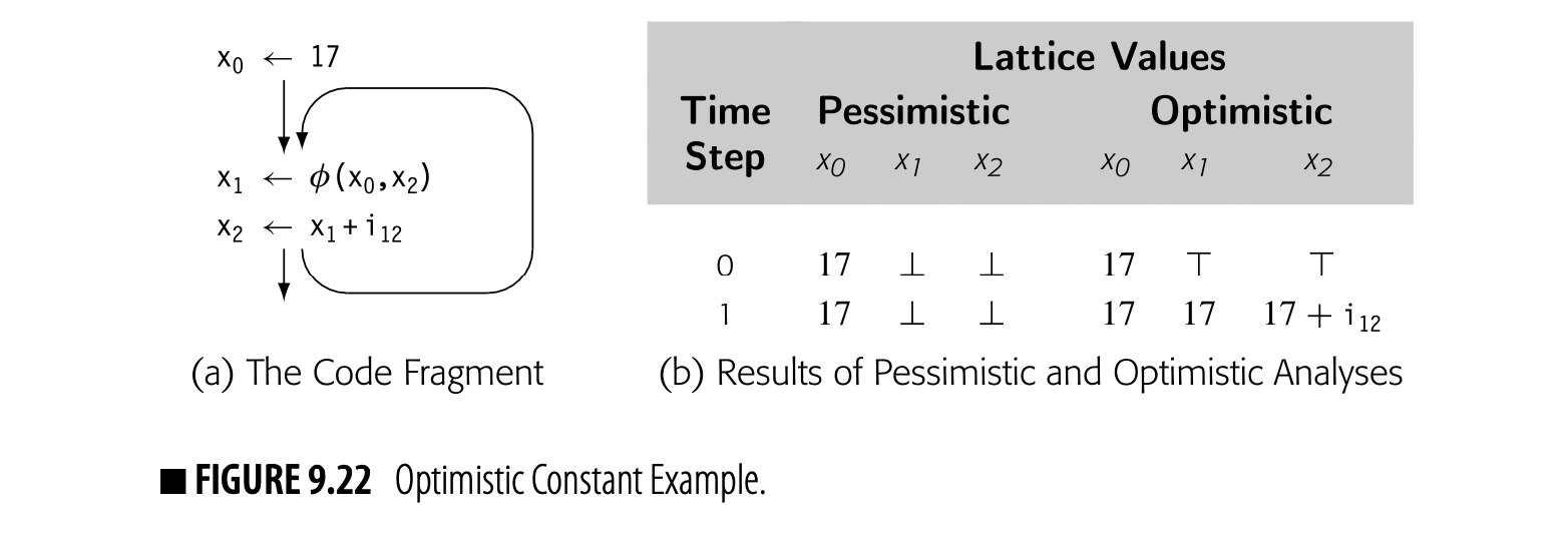
If, on the other hand, the algorithm initializes $x_1=\top$ and $x_2=\top$ (optimism), it can propagate $x_0$'s value into the loop. It computes $x_1$'s value as $17\wedge \top =17$. Since $x_1$'s value has changed, the algorithm places $x_1$ on WorkList. The algorithm then reevaluates the definition of $x_2$. If, for example, $i_{12}=0$, then $x_2$ gets the value $17$ and the algorithm adds $x_2$ to the worklist. When it reevaluates the $\varphi$-function, it sets $x_1=17\wedge 17=17$.

Consider what would happen if $i_{12}=2$, instead. Then, when SSCP evaluates $x_1+i_{12}$ it sets $x_2=19$. Next, it reevaluates $x_1=17\wedge 19=\perp$. This $\perp$, in turn, propagates to $x_2$, proving $x$ nonconstant in the loop.

The Value of SSA Form

The use of SSA form in SSCP leads to a simple and efficient algorithm. To see this point, consider a classic data-flow approach to the problem. It would create a set ConstantsIN at the top of each block and a set ConstantsOut at the end of each block. ConstantsIN and ConstantsOut would hold $⟨variable,value⟩$ pairs.

This sketch oversimplifies the algorithm. This formulation lacks a unique fixed point, so the results depend on the order in which the blocks are processed. It also lacks the properties that let the iterative algorithm converge quickly. Solvers may run in $O(n2$) time, or worse.

For a block $b$, the compiler could compute $ConstantsIN($b$)$ as a pairwise intersection of ConstantsOut($p$), taken over every $p\in preds(b)$. All the values for a single name would be intersected using the same meet function as in SSCP. To derive ConstantsOut($b$) from ConstantsIN($b$) the compiler could apply a version of LVN extended to handle $\perp$ and $\top$. An iterative fixed-point algorithm would halt when the sets stopped changing.

By contrast, SSCP is a simple iterative fixed-point algorithm operating on a sparse graph and particularly shallow lattice. It has the same complication with interpreting each operation over the known constant values, but it interprets single operations rather than whole blocks. It has an easily understood time bound. In this case, use of SSA form leads directly to a simple, efficient, sparse method for global constant propagation.

Section Review

SSA form encodes information about both data flow and control flow in a conceptually simple intermediate form. This section focused on the algorithms to translate code into and out of semipruned SSA form. The initial construction of SSA form is a two-step process. The first step inserts $\varphi$-functions into the code at join points where distinct definitions can converge. That algorithm relies on dominance frontiers for efficiency. The second step creates the SSA name space by adding subscripts to the original base names during a systematic traversal of the entire procedure.

Because processors do not directly implement $\varphi$-functions, the compiler must translate code out of SSA form before it can execute. Transformation of the code while in SSA form can complicate out-of-SSA translation. Section 9.3.5 examined both the "lost copy problem" and the "swap problem" and described approaches for handling them. Finally, Section 9.3.6 showed an algorithm for global constant propagation over the SSA-form.

Review Questions

1. Maximal SSA form includes useless $\varphi$-functions that define nonlive values and redundant $\varphi$-functions that merge identical values ($\text{e.g.},{\mathrm{x}}_8\leftarrow \varphi \left({\mathrm{x}}_7,{\mathrm{x}}_7\right))$. Can semipruned SSA insert nonlive or redundant $\varphi$-functions? If so, how can the compiler eliminate them?
2. Assume that your compiler targets an ISA that implements swap $r_1$, $r_2$, which simultaneously performs $r_1\leftarrow r_2$ and $r_2\leftarrow r_1$. What impact could swap have on out-of-SSA translation?

9.4 INTERPROCEDURAL ANALYSIS

Procedure calls introduce two kinds of inefficiencies: (1) loss of knowledge in single-procedure analysis and optimization because of a call site; and (2) overhead introduced to implement the abstractions inherent in procedure calls. Interprocedural analysis was introduced to address the former problem. We saw, in Section 9.2.4, that the compiler can compute sets that summarize each call site's side effects. This section explores more complex issues in interprocedural analysis.

9.4.1 Call-Graph Construction

The first problem that the compiler must address in interprocedural analysis is the construction of a call graph. In the simplest case, in whichevery procedure call invokes a procedure named by a literal constant, as in call fee(x,y,z), the problem is straightforward. The compiler creates a call-graph node for each procedure in the program and adds an edge to the call graph for each call site. This process takes time proportional to the number of procedures and the number of call sites in the program; in practice, the limiting factor will be the cost to locate the call sites.

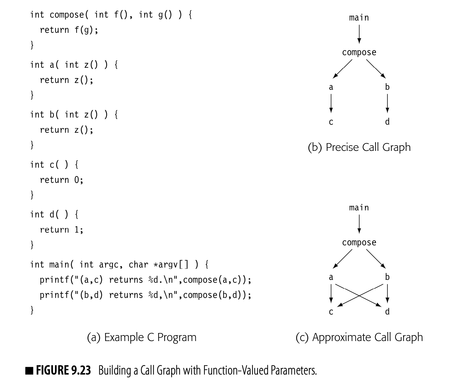
Source language features can complicate call-graph construction. For example, consider the small C program shown in Fig. 9.23(a). Its precise call graph is shown in panel (b). The following subsections outline the language features that complicate call-graph construction.

Procedure-Valued Variables

If the program uses procedure-valued variables, the compiler must either assume that a call to a procedure-valued variable can invoke any procedure, or it must analyze the program to estimate the set of possible callees at each such call site. To perform this analysis, the compiler can construct the graph specified by the calls that use explicit literal constants. Next, it can track the propagation of functions as values around this subset of the call graph, adding edges as indicated.

In SSCP, initialize any function-valued formal parameters with known constant values. Actual parameters with the known values reveal where functions are passed through.

The compiler can use a simple analog of global constant propagation to transfer function values from a procedure's entry to the call sites that use them, using set union as its meet operation.

Once it has a set of procedures that might be passed to a procedure-valued parameter, the compiler must model the transmission of that parameter to individual call sites in the procedure. Most programming languages do not allow operations on a procedure-value, so this modeling can be both simple and effective (see the discussion of jump functions in Section 9.4.2).

Fig. 9.23 shows that a straightforward analysis may overestimate the set of call-graph edges. The code calls compose to compute a(c) and b(d). A simple analysis, however, will conclude that the formal parameter g in compose can receive either c or d, and that, as a result, the program might compose any of a(c), a(d), b(c), or b(d), as shown in panel (c). To build the precise call graph, shown in panel (b), the compiler must track sets of parameters that are passed together, along the same path. The algorithm could then consider each set independently to derive the precise graph. Alternatively, it might tag each value with the path that the values travel and use the path information to avoid adding spurious edges such as (a,d) or (b,c).

Contextually Resolved Names

Some languages allow programmers to use names that are resolved by context. In object-oriented languages with an inheritance hierarchy, the binding of a method name to a specific implementation depends on the class of the receiver and the state of the inheritance hierarchy.

If the inheritance hierarchy and all the procedures are fixed at the time of analysis, then the compiler can use interprocedural analysis of the class structure to narrow the set of methods that can be invoked at any given call site. The call-graph constructor must include an edge from that call site to each procedure or method that might be invoked.

Dynamic linking, used in some operating systems to reduce virtual memory require- ments, introduces similar complications. If the compiler cannot determine what code will execute, it cannot construct a complete call graph.

For a language that allows the program to import either executable code or new class definitions at runtime, the compiler must construct a conservative call graph that reflects the complete set of potential callees at each call site. One option is to have the compiler construct a single call-graph node to represent these unknown procedures and to endow that node with worst-case behavior, such as maximal MayMod and MayRef sets. This strategy will ensure that other analyses have conservative approximations to the set of possible facts.

Analysis to resolve ambiguous calls can improve the precision of the call graph by reducing the number of spurious edges--edges for calls that cannot occur at runtime. Of equal or greater importance, any call site that can be resolved to a single callee can be implemented with a direct call; one with multiple callees may need a runtime lookup to dispatch the call (see Section 6.3.2). Runtime lookups to support dynamic dispatch can be much more expensive than a direct call.

Other Language Issues

In intraprocedural analysis, we assume that the control-flow graph has a single entry and a single exit; we add an artificial exit node if the procedure has multiple returns. The analogous problems arise in interprocedural analysis.

For example, JAVA has both initializers and finalizers. The JAVA virtual machine invokes a class initializer after it loads and verifies the class; it invokes an object initializer after it allocates space for the object but before it returns the object's hashcode. Thread start methods, finalizers, and destructors also have the property that they execute without an explicit call in the source program.

The call-graph builder must recognize and understand these procedures. It must connect them into the call graph in appropriate ways. The specific details will depend on the language definition and the analysis being performed. MayMod analysis, for example, might ignore them as irrelevant, while interprocedural constant propagation might need information from initialization and start methods.

9.4.2 Interprocedural Constant Propagation

Interprocedural constant propagation tracks known constant values of global variables and parameters as they propagate around the call graph, both through procedure bodies and across call-graph edges. The goal of interprocedural constant propagation is to discover places where a procedure always receives a known constant value or where a procedure always returns a known constant value. When the compiler finds such a constant, it can specialize the code to that value.

For the moment, we will restrict our attention to finding constant-valued formal parameters. The extension to global variables appears at the end of this section.

Conceptually, interprocedural constant propagation consists of three sub-problems: discovering an initial set of constants, propagating known constant values around the call graph, and modeling transmission of values through procedures.

Discovering an Initial Set of Constants

The analyzer must identify, at each call site, which actual parameters have known constant values. A wide range of techniques are possible. The simplest method is to recognize literal constant values used as parameters. A more effective and expensive approach could use global constant propagation (e.g., SSCP from Section 9.3.6) to identify constant-valued parameters.

Propagating Known Constant Values Around the Call Graph

Given an initial set of constants, the analyzer propagates the constant values across call-graph edges and through the procedures from entry to each call site in the procedure. This portion of the analysis resembles the iterative data-flow algorithms from Section 9.2. The iterative algorithm will solve this problem, but it may require significantly more iterations than it would for simpler problems such as live variables or available expressions.

Modeling Transmission of Values Through Procedures

Each time the analyzer processes a call-graph node, it must determine how the constant values known at the procedure's entry affect the set of constant values known at each of the call sites in the procedure. To do so, it builds a small model for each actual parameter, called a jump function. At a call site $s$, we will denote the jump function for parameter $a$ as ${\mathcal{J}}_s^a$.

Each call site $s$ is represented with a vector of jump functions. If $s$ has $n$ parameters, the algorithm builds the vector ${\mathcal{J}}_s=⟨{\mathcal{J}}_s^a,{\mathcal{J}}_s^b,{\mathcal{J}}_s^c,\dots ,{\mathcal{J}}_s^n⟩$, where $a$ is the first formal parameter in the callee, $b$ is the second, and so on. Each jump function, ${\mathcal{J}}_s^x$, relies on the values of some subset of the global variables and the formal parameters to the procedure $p$ that contains $s$; we denote that set as Support(${\mathcal{J}}_s^x$).

For the moment, assume that ${\mathcal{J}}_s^x$ consists of an expression tree whose leaves are all global variables, formal parameters of the caller, or literal constants. We require that ${\mathcal{J}}_s^x$ return $\top$ if Value(y) is $\top$ for any $y\in \text{Support}({\mathcal{J}}_s^x)$.

The Algorithm

Fig. 9.24 shows a simple interprocedural constant propagation algorithm. It is similar to the SSCP algorithm presented in Section 9.3.6.

The algorithm associates a field Value($x$) with each formal parameter $x$ of each procedure $p$. (It assumes unique, or fully qualified, names for each formal parameter.) The first phase optimistically sets all the Value fields to $\top$. Next, it iterates over each actual parameter $a$ at each call site $s$ in the program, updates the Value field of $a$'s corresponding formal parameter $f$ to $Value(f)\wedge {\mathcal{J}}_s^f$, and adds $f$ to the worklist. This step factors the initial set of constants represented by the jump functions into the $Value$ fields and sets the worklist to contain all of the formal parameters.

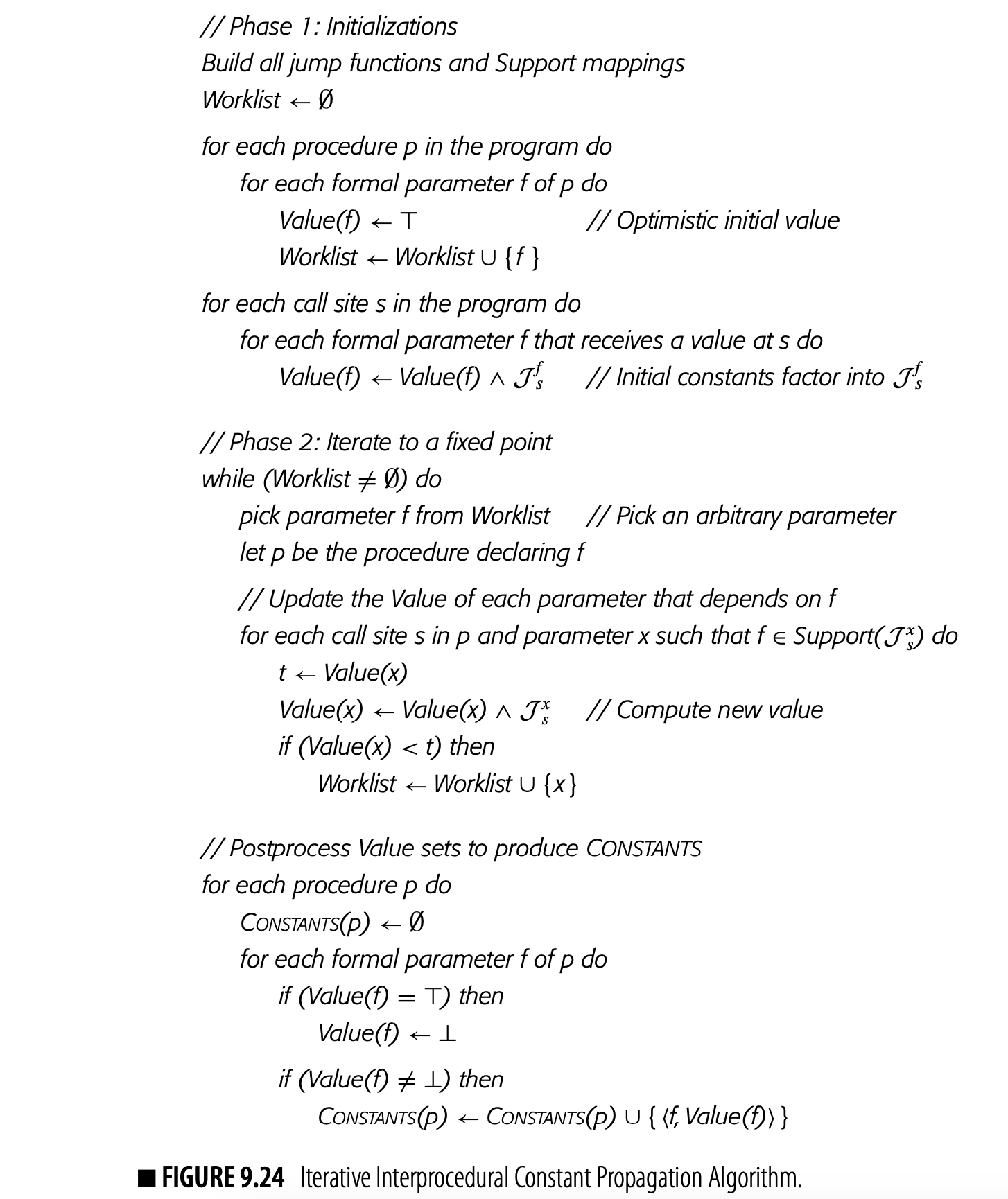
The second phase repeatedly selects a formal parameter from the worklist and propagates it. To propagate formal parameter $f$ of procedure $p$, the analyzer finds each call site $s$ in $p$ and each formal parameter $x$ (which corresponds to an actual parameter of call site $s$) such that $f\in Support({\mathcal{J}}_s^x)$. It evaluates ${\mathcal{J}}_s^x$ and combines it with $Value(x)$. If $Value(x)$ changes, it adds $x$ to the worklist. The worklist should be implemented with a data structure, such as a sparse set, that does not allow duplicate members (see Section B.2.3).

This algorithm relies on the same semilattice-based termination argument used for SSCP in Section 9.3.6.

The second phase terminates because each Value set can take on at most three values in the semilattice: $\top$, some $c_i$, and $\perp$. A variable $x$ can only enter the worklist when its initial Value is computed or when its Value changes. Each variable $x$ can appear on the worklist at most three times. Thus, the total number of changes is bounded and the iteration halts. After the second phase halts, a postprocessing step constructs the sets of constants known on entry to each procedure.

Jump Function Implementation

For example, $\mathrm{Support}\left({\mathcal{J}}_s^x\right)$ might contain a value read from a file, so ${\mathcal{J}}_s^x=\perp$.

Implementations of jump functions range from simple static approximations that do not change during analysis, through small parameterized models, to more complex schemes that perform extensive analysis at each jump-function evaluation. In any of these schemes, several principles hold. If the analyzer determines that parameter $x$ at call site $s$ is a known constant $c$, then ${\mathcal{J}}_s^x=c$ and $\text{Support}({\mathcal{J}}_s^x)=\varnothing$. If $y\in \text{Support}({\mathcal{J}}_s^x)$ and $\text{Value}(y)=\top$, then ${\mathcal{J}}_s^x=\top$. If the analyzer determines that the value of ${\mathcal{J}}_s^x$ cannot be determined, then ${\mathcal{J}}_s^x=\perp$.

The analyzer can implement ${\mathcal{J}}_s^x$ in many ways. A simple implementation might only propagate a constant if the value enters the procedure as a formal parameter and passes, unchanged, to a parameter at a call site--that is, an actual parameter $x$ is the SSA name of a formal parameter in the procedure that contains call site $s$. (Similar functionality can be obtained using Reaches information from Section 9.2.4.)

More complex schemes that find more constants are possible. The compiler could build expressions composed of SSA names of formal parameters and literal constants. The jump-function would then interpret the expression over the semilattice values of the SSA names and constants that it contains. To obtain even more precise results, the compiler could run the SSCP algorithm on demand to update the values of jump functions.

Extending the Algorithm

The algorithm shown in Fig. 9.24 only propagates constant-valued actual parameters forward along call-graph edges. We can extend it, in a natural way, to handle returned values and variables that are global to a procedure.

Just as the algorithm builds jump functions to model the flow of values from caller to callee, it can construct return jump functions to model the values returned from callee to caller. Return jump functions are particularly important for routines that initialize values, whether filling in a common block in FORTRAN or setting initial values for an object or class in JAVA. The algorithm can treat return jump functions in the same way that it handled ordinary jump functions; the one significant complication is that the implementation must avoid creating cycles of return jump functions that diverge (e.g., for a tail-recursive procedure).

To extend the algorithm to cover a larger class of variables, the compiler can extend the vector of jump functions in an appropriate way. Expanding the set of variables will increase the cost of analysis, but two factors mitigate the cost. First, in jump-function construction, the analyzer can notice that many of those variables do not have a value that can be modeled easily; it can map those variables onto a universal jump function that returns $\perp$ and avoid placing them on the worklist. Second, for the variables that might have constant values, the structure of the lattice ensures that they will be on the worklist at most twice. Thus, the algorithm should still run quickly.

Section Review

Compilers perform interprocedural analysis to capture the behavior of all the procedures in the program and to bring that knowledge to bear on optimization within individual procedures. To perform interprocedural analysis, the compiler must model all of the code that it analyzes. A typical interprocedural problem requires the compiler to build a call graph (or some analog), to annotate it with information derived directly from the individual procedures, and to propagate that information around the graph.

The results of interprocedural information are applied directly in intraprocedural analysis and optimization. For example, MarMood and MarRer sets can be used to mitigate the impact of a call site on global data-flow analyses or to avoid the necessity for $\mathbf{\varphi }$-functions after a call site. The results of interprocedural constant propagation can be used to initialize a global algorithm, such as sparse conditional constant propagation (see Section 0.1.7).

Review Questions

1. Call-graph construction has many similarities to interprocedural constant propagation. The call-graph algorithm can achieve good results with relatively simple jump functions. What features could a language designer add that might necessitate more complex jump functions in the call-graph constructor?
2. How might the analyzer incorporate MarMood information into interprocedural constant propagation? What effect would you expect it to have?

9.5 Advanced Topics

Section 9.2 focused on iterative data-flow analysis. It emphasized the iterative approach because it is simple, robust, and efficient. Other approaches to data-flow analysis tend to rely heavily on structural properties of the underlying graph. Section 9.5 discusses flow-graph reducibility--a critical property for most of the structural algorithms.

Section 9.5.2 revisits the iterative dominance framework from Section 9.2.1. The simplicity of that framework makes it attractive; however, more specialized and complex algorithms have significantly lower asymptotic complexities. In Section 9.5.2, we introduce a set of data structures that make the simple iterative technique competitive with the fast dominator algorithms for flow graphs of up to several thousand nodes.

9.5.1 Structural Data-Flow Analysis and Reducibility

Chapters 8 and 9 present an iterative formulation of data-flow analysis. The iterative algorithm works, in general, on any set of well-formed equations on any graph. Other data-flow algorithms exist; many of these work by deriving a simple model of the control-flow structure of the code being analyzed and using that model to solve the equations. Often, that model is built by finding a sequence of transformations to the CFG that reduce its complexity--by combining nodes or edges in carefully defined ways. This graph-reduction process lies at the heart of almost every data-flow algorithm except the iterative algorithm.

Reducible graph A flow graph is reducible if the two transformations, $T_1$ and $T_2$, will reduce it to a single node. If that process fails, the graph is $\text{irreducible}$.

These $structural$ data-flow algorithms use a small set of transformations, each of which selects a subgraph and replaces it by a single node to represent the subgraph. This creates a series of derived graphs in which each graph differs from its predecessor in the series by the effect of applying a single transformation. As the analyzer transforms the graph, it computes data-flow sets for the new representer nodes in each successive derived graph. These sets summarize the replaced subgraph's effects. The transformations reduce well-behaved graphs to a single node. The algorithm then reverses the process, going from the final derived graph, with its single node, back to the original flow graph. As it expands the graph back to its original form, the analyzer computes the final data-flow sets for each node.

In essence, the reduction phase gathers information from the entire graph and consolidates it, while the expansion phase propagates the effects in the consolidated set back out to the nodes of the original graph. Any graph for which such a reduction sequence succeeds is deemed reducible. If the graph cannot be reduced to a single node, it is irreducible. 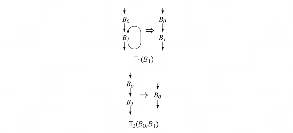To demonstrate reducibility, we can use the two graph transformations, called $T_1$ and $T_2$, shown in the margin. These same transformations form the basis for a classic data-flow algorithm. $T_1$ removes a self loop, which is an edge that runs from a node back to itself. The drawing in the margin shows $T_1$ applied to $B_I$, denoted $T_1(B_I)$. $T_2$ folds a node $B_I$ that has exactly one predecessor $B_0$ back into $B_0$; it removes the edge $⟨B_0,B_I⟩$, and makes $B_0$ the source of any edges that originally left $B_I$. If this leaves multiple edges from $B_0$ to some other node $n$, it consolidates those edges. The drawing in the margin shows $T_2(B_0,B_I)$.

Any graph that can be transformed, or reduced, to a single node by repeated application of $T_1$ and $T_2$ is deemed reducible. To understand how this works, consider the CFG from our continuing example. Fig. 9.25(a) shows one sequence of applications of $T_1$ and $T_2$ that reduces the CFG to a single-node graph. The sequence applies $T_2$ until no more opportunities exist: $T_2(B_I,B_2)$, $T_2(B_5,B_6)$, $T_2(B_5,B_8)$, $T_2(B_5,B_7)$, $T_2(B_I,B_5)$, and $T_2(B_I,B_3)$. Next, it uses $T_1(B_I)$ to remove the loop. Finally, it applies $T_2(B_0,B_I)$ and $T_2(B_0,B_4)$ to reduce the graph to a single node. This sequence proves that the graph is reducible.

Other application orders also reduce the graph. For example, starting with $T_2(B_I,B_3)$ leads to a different transformation sequence. $T_1$ and $T_2$ have the finite Church-Rosser property, which ensures that the final result is independent of the order of application and that the sequence terminates. Thus, the analyzer can find places in the graph where $T_1$ or $T_2$ applies and use them opportunistically.

Fig. 9.25(b) shows what can happen when we apply $T_1$ and $T_2$ to a graph with multiple-entry loops. The analyzer uses $T_2(B_0,B_I)$ followed by $T_2(B_0,B_5)$. At that point, however, no remaining node or pair of nodes is a candidate for either $T_1$ or $T_2$. Thus, the analyzer cannot reduce the graph any further. (No other order will work either.) The graph cannot be reduced to a single node; it is irreducible.

Many other tests for graph reducibility exist. One fast and simple test is to apply the iterative DOM framework to the graph, using an RPO traversal order. If the calculation needs more than two iterations over a graph, that graph is irreducible.

The failure of $T_1$ and $T_2$ to reduce this graph arises from a fundamental property of the graph. The graph is irreducible because it contains a loop, or cycle, that has edges that enter it at different nodes. In terms of the source language, the program that generated the graph has a loop with multiple entries. We can see this property in the graph; consider the cycle formed by $B_2$ and $B_3$. It has edges entering it from $B_I$, $B_4$, and $B_5$. Similarly, the cycle formed by $B_3$ and $B_4$ has edges that enter it from $B_2$ and $B_5$.

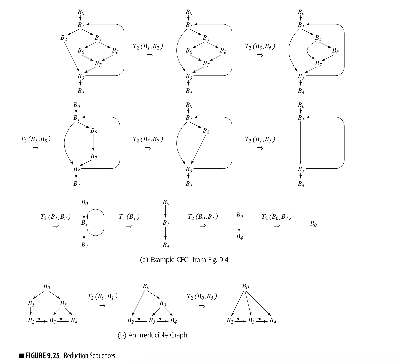
Irreducibility poses a serious problem for algorithms built on transformations like $T_1$ and $T_2$. If the algorithm cannot reduce the graph to a single-node, then the method must either report failure, modify the graph by splitting one or more nodes, or use an iterative approach to solve the system on the partially reduced graph. In general, structural algorithms for data-flow analysis only work on reducible graphs. The iterative algorithm, by contrast, works correctly, albeit more slowly, on an irreducible graph. 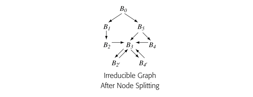To transform an irreducible graph to a reducible graph, the analyzer can split one or more nodes. The simplest split for the example graph from Fig. 9.25(b) is shown in the margin. The transformation has cloned $B_2$ and $B_d$ to create $B_{2^{\prime }}$ and $B_{d^{\prime }}$, respectively. The analyzer then retargets the edges$(B_3,B_2)$ and $(B_3,B_4)$ to form a complex loop, $\{B_3,B_{2^{\prime }},B_{4^{\prime }}\}$. The new loop has a single entry, through $B_3$.

This transformation creates a reducible graph that executes the same sequence of operations as the original graph. Paths that, in the original graph, entered $B_3$ from either $B_2$ or $B_4$ now execute as prologs to the loop $\{B_3,B_{2^{\prime }},B_{4^{\prime }}\}$. Both $B_2$ and $B_4$ have unique predecessors in the new graph. $B_3$ has multiple predecessors, but it is the sole entry to the loop and the loop is reducible. Thus, node splitting produced a reducible graph, at the cost of cloning two nodes.

In the reverse CFG, the break becomes a second entry to the cyclic region.

Both folklore and published studies suggest that irreducible graphs rarely arise in global data-flow analysis. The rise of structured programming in the 1970s made programmers much less likely to use arbitrary transfers of control, like a goto statement. Structured loop constructs, such as do, for, while, and until loops, cannot produce irreducible graphs. However, transferring control out of a loop (for example, C's break statement) creates a CFG that is irreducible to a backward analysis. Similarly, irreducible graphs may arise more often in interprocedural analysis due to mutually recursive subroutines. For example, the call graph of a recursive-descent parser is likely to have irreducible subgraphs. Fortunately, an iterative analyzer can handle irreducible graphs correctly and efficiently.

A simple way to avoid worst case behavior from an irreducible graph in an iterative analyzer is to compute two traversal orders, one based on the treewalk that traverses siblings left-to-right and another based on a right-to-left traversal. Alternating between these two orders on successive passes will improve behavior on worst-case irreducible graphs.

9.5.2 Speeding up the Iterative Dominance Framework

The iterative framework for computing dominance is particularly simple. Where most data-flow problems have equations involving several sets, the equations for Dom involve computing a pairwise intersection over Dom sets and adding a single element to those sets. The simple nature of these equations presents an opportunity; we can use a sparse data-structure to improve the speed of the $\text{Dom}$ calculation.

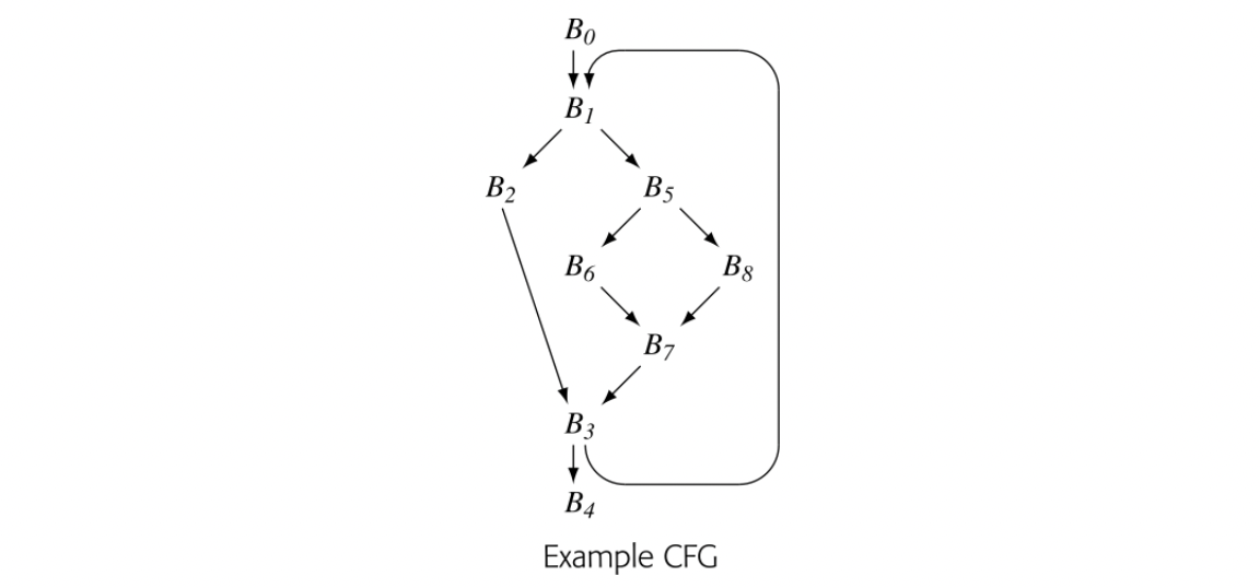
The iterative Dom framework described in Section 9.2.1 stores a full Dom set at each node. The compiler can achieve the same result by storing just the immediate dominator, or IDom, at each node and solving for IDom. The compiler can easily recreate Dom($n$) when needed. Since IDom is a singleton set, the implementation can be quite efficient.

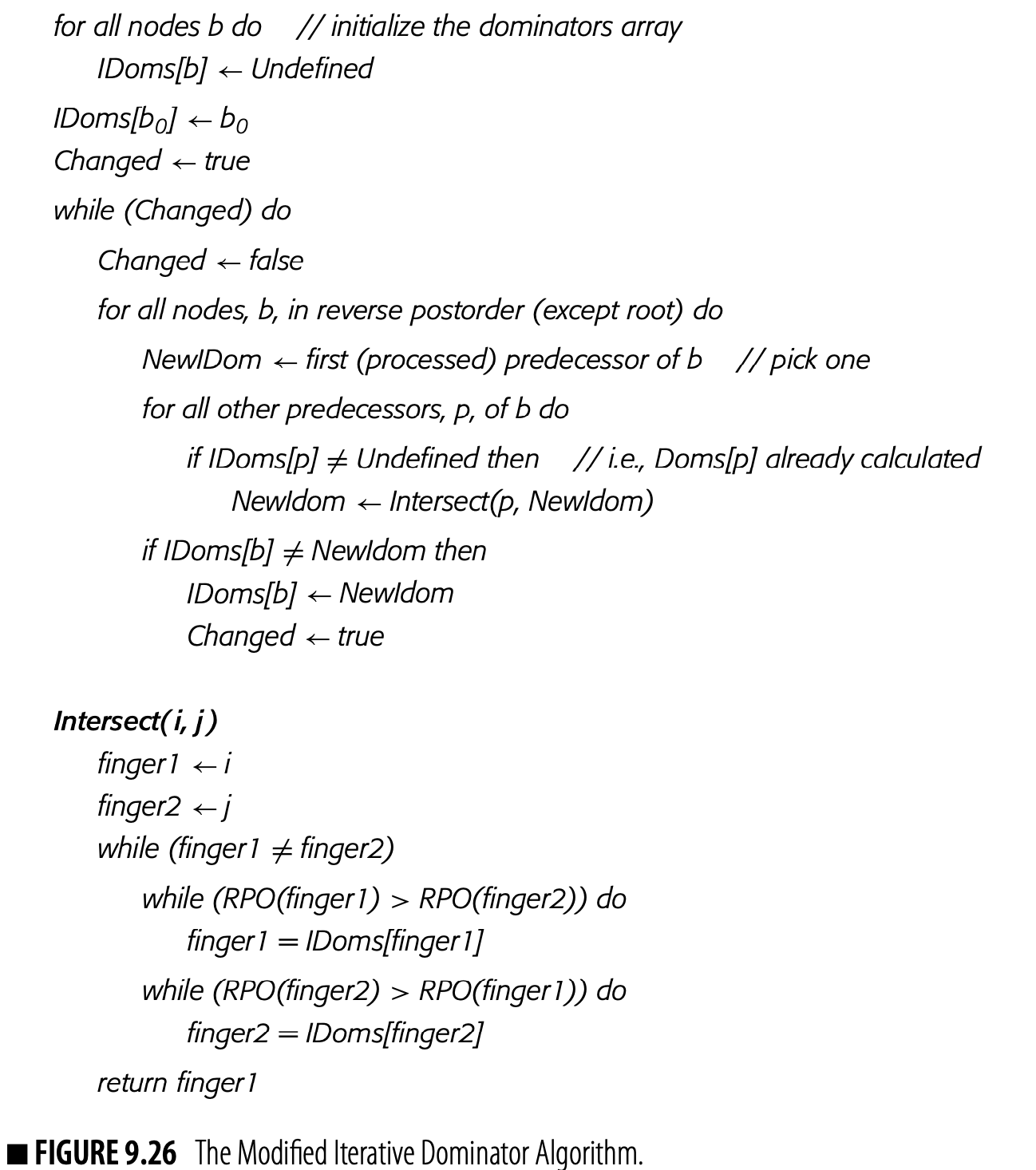
Recall our example CFG from Section 9.2.1, repeated in the margins along with its dominator tree. Its IDom sets are as follows:

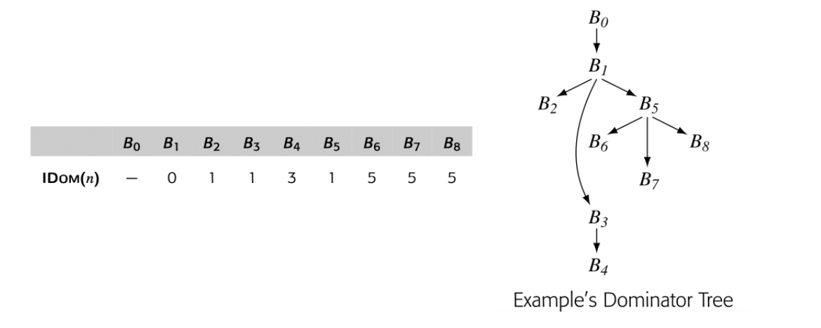
Notice that the dominator tree and the IDoms are isomorphic. IDom($b$) is just $b$'s predecessor in the dominator tree. The root of the dominator tree has no predecessor; accordingly, its IDom set is undefined.

The compiler can read a graph's Dom sets from its dominator tree. For a node $n$, its Dom set is just the set of nodes that lie on the path from $n$ to the root of the dominator tree, inclusive of the end points. In the example, the dominator-tree path from $B_7$ to $B_0$ consists of $(B_7,B_5,B_1,B_0)$, which matches Dom($B_7$) from Section 9.2.1.

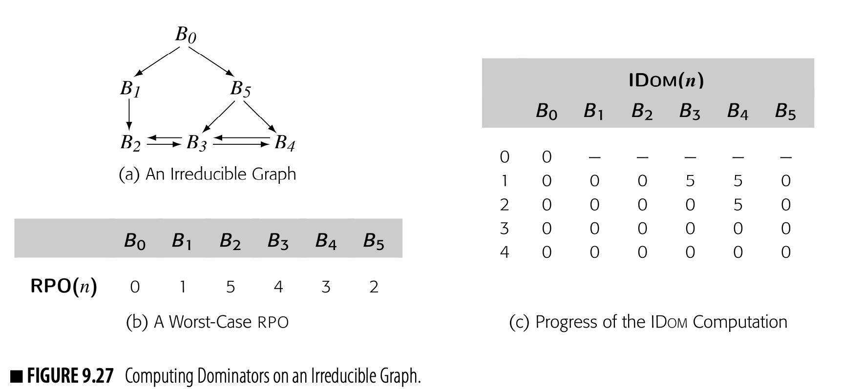
Thus, the compiler can use the IDom sets as a proxy for the Dom sets, provided that it can initialize and intersect the sets efficiently. A small modification to the iterative algorithm can simplify initialization. Intersection requires a more subtle approach, shown in Fig. 9.26. The critical procedure, intersect, relies on two observations:

1. When the algorithm walks the path from a node to the root to recreate a Dom set, it encounters the nodes in a consistent order. The intersection of two Dom sets is simply the common suffix of the labels on the paths from the nodes to the root.
2. The algorithm needs to recognize the common suffix. It starts at the two nodes whose sets are being intersected, $i$ and $j$, and walks upward in the dominator tree from each of them toward the root. If we name the nodes by their RPO numbers, then a simple comparison will let the algorithm discover the nearest common ancestor--the IDom of $i$ and $j$.

intersect is a variant of the classic "two finger" algorithm. It uses two pointers to trace paths upward through the tree. When they agree, they both point to the node representing the result of the intersection.

Fig. 9.26 shows a reformulated iterative algorithm for IDom. It keeps the IDom information in an array, IDoms. It initializes the IDom entry for the root, b${}_0$, to itself to simplify the rest of the algorithm. It processes the nodes in reverse postorder. In computing intersections, it ignores predecessors whose IDoms have not yet been computed.

To see how the algorithm operates, consider the irreducible graph in Fig. 9.27(a). Panel (b) shows an RPO for this graph that illustrates the problems caused by irreducibility. Using this order, the algorithm miscomputes the IDoms of $B_3$, and $B_4$ in the first iteration. It takes two iterations for thealgorithm to correct those IDoms, and a final iteration to recognize that the IDoms have stopped changing.

This improved algorithm runs quickly. It has a small memory footprint. On any reducible graph, it halts in two passes: the first pass computes the correct IDom sets and the second pass confirms that no changes occur. An irreducible graph will take more than two passes. In fact, the algorithm provides a rapid test for reducibility--if any IDom entry changes in the second pass, the graph is irreducible.

9.6 Summary and Perspective

Most optimization tailors general-case code to the specific context that occurs in the compiled code. The compiler's ability to tailor code is often limited by its lack of knowledge about the program's range of runtime behaviors.

Data-flow analysis allows the compiler to model the runtime behavior of a program at compile time and to draw important, specific knowledge from these models. Many data-flow problems have been proposed; this chapter presented several of them. Many of those problems have properties that lead to efficient analyses.

SSA form is both an intermediate form and a tool for analysis. It encodes both data-flow information and control-dependence information into the name space of the program. Using SSA form as the basis for an algorithm has three potential benefits. It can lead to more precise analysis, because SSA incorporates control-flow information. It can lead to more efficient algorithms, because SSA is a sparse representation for the underlying data-flow information. It can lead to simpler formulations of the underlying optimization (see Section 10.7.2). These advantages have led both researchers and practitioners to adopt SSA form as a definitive representation in modern compilers.

Chapter Notes

Credit for the first data-flow analysis is usually given to Vyssotsky at Bell Labs in the early 1960s [351]. Lois Haibt's work, in the original FORTRAN compiler, predates Vyssotsky. Her phase of the compiler built a control-flow graph and performed a Markov-style analysis over the CFG to estimate execution frequencies [27].

Iterative data-flow analysis has a long history in the literature. Among the seminal papers on this topic are Kildall's 1973 paper [234], work by Hechtand Ullman [197], and two papers by Kam and Ullman [221, 222]. The treatment in this chapter follows Kam & Ullman.

This chapter focuses on iterative data-flow analysis. Many other algorithms for solving data-flow problems have been proposed [229]. The interested reader should explore the structural techniques, including interval analysis [18, 19, 68]; $T_1$-$T_2$ analysis [196, 348]; the Graham-Wegman algorithm [178, 179]; the balanced-tree, path-compression algorithm [342, 343]; graph grammars [230]; and the partitioned-variable technique [371]. The alternating-direction iterative method mentioned at the end of Section 9.5.1 is due to Harvey [109].

Dominance has a long history in the literature. Prosser introduced dominance in 1959 but gave no algorithm to compute dominators [300]. Lowry and Medlock describe the algorithm used in their compiler [260]; it takes at least \mathsf{O}\big{(}N^{2}\big{)} time, where $N$ is the number of statements in the procedure. Several authors developed faster algorithms based on removing nodes from the cfg[4, 9, 301]. Tarjan proposed an $\mathsf{O}(N\log N+E)$ algorithm based on depth-first search and union find [341]. Lengauer and Tarjan improved this time bound [252], as did others [24, 67, 190]. The data-flow formulation for dominators is taken from Allen [13, 18]. The fast data structures for iterative dominance are due to Harvey [110]. The algorithm in Fig. 9.10 is from Ferrante, Ottenstein, and Warren [155].

The SSA construction is based on the seminal work by Cytron et al. [120]. That work builds on work by Shapiro and Saint [323]; by Reif [305, 344]; and by Ferrante, Ottenstein, and Warren [155]. The algorithm in Section 9.3.3 builds semipruned SSA[55]. Briggs et al. describe the details of the renaming algorithm and the ad-hoc approach to out-of-SSA translation [56]. The unified approach to out-of-SSA translation is due to Boissinot et al. [51]. The complications introduced by critical edges have long been recognized in the literature of optimization [139, 141, 142, 236, 312]; it should not be surprising that they also arise in the translation from SSA back into executable code. The sparse simple constant algorithm, SSCP, is due to Reif and Lewis [306]. Wegman and Zadeck reformulate SSCP to use SSA form [358, 359].

The IBM PL/I optimizing compiler was one of the earliest systems to perform interprocedural data-flow analysis [334]. Call-graph construction is heavily language dependent: Ryder looked at the problems that arise in Fortran [314], C [272], and JAVA[372]. Shivers wrote the classic paper on control-flow analysis in Scheme-like languages [325].

Early work on side-effect analysis focused more on defining the problems than on their fast solution [35, 37]. Cooper and Kennedy developed simple frameworks for MayMod and MayRef that led to fast algorithms for these problems [112, 113]. The interprocedural constant propagation algorithm is from Torczon's thesis and subsequent papers [74, 182, 271]; both Cytron and Wegman suggested other approaches to the problem [121, 359]. Burke and Torczon [70] formulated an analysis that determines which modules in a large program must be recompiled in response to a change in a program's interprocedural information. Pointer analysis is inherently interprocedural; a growing body of literature describes that problem [84, 87, 123, 134, 149, 202, 203, 209, 247, 322, 360, 363]. Ayers, Gottlieb, and Schooler described a practical system that analyzed and optimized a subset of the entire program [26].

Exercises

1. In live analysis, the equations initialize the LiveOut set of each block to $\varnothing$. Are other initializations possible? Do they change the result of the analysis? Justify your answer.

2. In live analysis, how should the compiler treat a block containing a procedure call? What should the block's UEVar set contain? What should its VarKill set contain?

3. For each of the following control-flow graphs: a. Compute reverse postorder numberings for the CFG and the reverse CFG. b. Compute reverse preorder on the CFG. c. Is reverse preorder on the CFG equivalent to postorder on the reverse CFG?

   • Consider the three control-flow graphs shown in Fig. 9.28.
   • Compute the dominator trees for CFGs (a), (b), and (c).
   • Compute the dominance frontiers for nodes 3 and 5 of (a), nodes 4 and 5 of (b), and nodes 2 and 10 of (c).
   • Translate the code in the cfg shown below into SSA form. Show only the final results, after both $\varphi$-insertion and renaming.

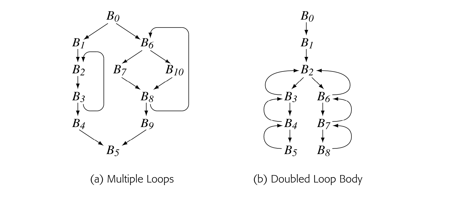
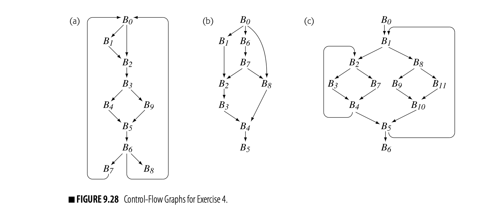
4. Consider the three control-flow graphs shown in Fig. 9.28.

   1. Compute the dominator trees for CFGs (a), (b), and (c).
   2. Compute the dominance frontiers for nodes 3 and 5 of (a), nodes 4 and 5 of (b), and nodes 2 and 10 of (c).

5. Translate the code in the CFG shown below into SSA form. Show only the final results, after both φ-insertion and renaming.

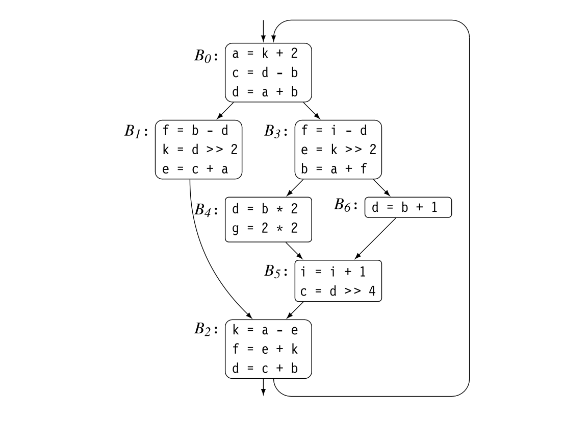
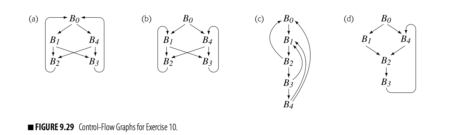
6. Given an assignment to some variable $v$ in block $b$, consider the set of blocks that need a $\varphi$-function as a result. The algorithm in Fig. 9.11 inserts a $\varphi$-function in each block in $\mathrm{DF}(b)$. It then adds each of those blocks to the worklist; they, in turn, may add more blocks to the worklist. Call the set of all these blocks ${\mathrm{DF}}^{+}(b)$. We can define ${\mathrm{DF}}^{+}(b)$ as the limit of the sequence: 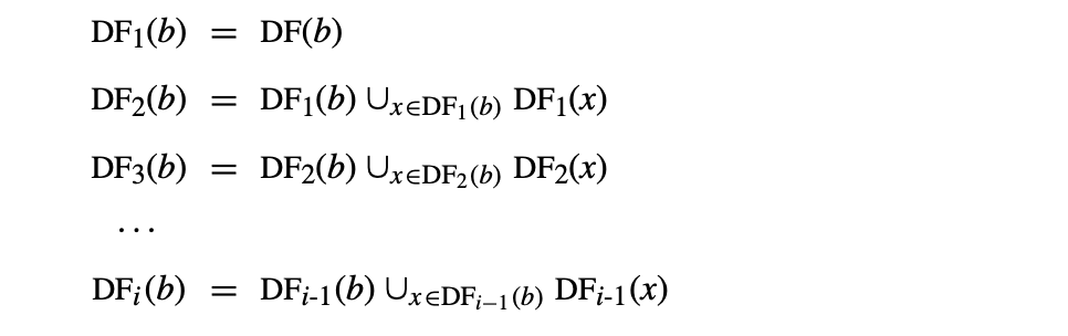Using these extended sets, ${\mathrm{DF}}^{+}(b)$, leads to a simpler algorithm for inserting $\varphi$-functions. a. Develop an algorithm to compute ${\mathrm{DF}}^{+}(b)$. b. Develop an algorithm to insert $\varphi$-functions using the ${\mathrm{DF}}^{+}$ sets computed in part (a). c. Compare the overall cost of your algorithm, including the computation of ${\mathrm{DF}}^{+}$ sets, to the cost of the $\varphi$-insertion algorithm given in Section 9.3.3.

7. The maximal SSA construction is both simple and intuitive. However, it can insert many more $\varphi$-functions than the semipruned algorithm. In particular, it can insert both redundant $\varphi$-functions (${\mathrm{x}}_1\leftarrow \varphi ({\mathrm{x}}_j,{\mathrm{x}}_j)$) and dead $\varphi$-functions--functions whose results are never used. a. Propose a method to detect and remove the extra $\varphi$-functions that the maximal construction inserts. b. Can your method reduce the set of $\varphi$-functions to just those that the semipruned construction inserts? c. Contrast the asymptotic complexity of your method against that of the semipruned construction.

8. Apply the unified out-of-SSA translation scheme to the example code for the lost-copy problem, shown in Fig. 9.18(a).

9. Apply the unified out-of-SSA translation scheme to the example code for the swap problem, shown in Fig. 9.19(a).

10. For each of the control-flow graphs shown in Fig. 9.29, show whether or not it is reducible. (Hint: use a sequence of $T_1$ and $T_2$ to show that the graph is reducible. If no such sequence exists, it is irreducible.)

11. Prove that the following definition of a reducible graph is equivalent to the definition that uses the transformations $T_1$ and $T_2$: "A graph $G$ is reducible if and only if for each cycle in $G$, there exists a node $n$ in the cycle with the property that $n$ dominates every node in that cycle."